The Data Science Lab
Gaussian Mixture Model Data Clustering from Scratch Using C#
Data clustering is the process of grouping data items so that similar items are placed in the same cluster. There are several different clustering techniques, and each technique has many variations. Common clustering techniques include k-means, Gaussian mixture model, density-based and spectral. This article explains how to implement Gaussian mixture model (GMM) clustering from scratch using the C# programming language.
Compared to other clustering techniques, GMM clustering gives the pseudo-probabilities of cluster membership, as opposed to just assigning each data item to a single cluster ID. For example, if there are k = 3 clusters, a particular data item might have cluster pseudo-probabilities [0.15, 0.10, 0.85], which indicates the item most likely belongs to cluster ID = 2. However, compared to other techniques, GMM clustering is more complex to implement and a bit more complicated to interpret.
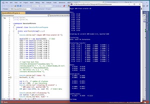
A good way to see where this article is headed is to take a look at the screenshot of a demo program in Figure 1. For simplicity, the demo uses just N = 10 data items:
0.01, 0.10
0.02, 0.09
0.03, 0.10
0.04, 0.06
0.05, 0.06
0.06, 0.05
0.07, 0.05
0.08, 0.01
0.09, 0.02
0.10, 0.01
Each data item is a vector with dim = 2 elements. GMM clustering is designed for strictly numeric data. After GMM with k = 3 clusters is applied to the data, the resulting clustering is: (1, 1, 2, 0, 1, 1, 0, 2, 1, 1). This means data item [0] is assigned to cluster 1, item [1] is assigned to cluster 1, item [2] is assigned to cluster 2, item [3] is assigned to cluster 0 and so on.
Behind the scenes, each of the three clusters has a mean, a 2-by-2 covariance matrix, and a coefficient (sometimes called a weight). The means, covariance matrices and coefficients are used to compute the cluster IDs.
 [Click on image for larger view.] Figure 1: Gaussian Mixture Model Data Clustering in Action
The demo program displays the three cluster means, all of which are [0.550, 0.550]. The three means are the same because there are so few data items. In a non-demo scenario the cluster means will usually be different. GMM clustering is not well-suited for very small or extremely large datasets.
This article assumes you have intermediate or better programming skill but doesn't assume you know anything about Gaussian mixture model clustering. The demo is implemented using C#. Because of the underlying mathematical complexity of GMM, refactoring the demo code to another C-family language is feasible but will require significant effort.
The source code for the demo program is too long to be presented in its entirety in this article. The complete code is available in the accompanying file download. The demo code and data are also available online.
Understanding Gaussian Mixture Model Clustering
One of the keys to GMM clustering is understanding multivariate Gaussian distributions. Suppose you are looking at the heights of a large group of the men. If you create a bar graph of the frequencies of height data it will have a bell-shaped curve with a mean like 68.00 inches and variance (a measure of spread) like 9.00 inches-squared. The total area of the bars will be 1.00.
A Gaussian distribution is a mathematical abstraction where the graph is a smooth curve instead of a collection of bars. A Gaussian distribution is completely characterized by a mean and a variance (or equivalently, a standard deviation which is just the square root of the variance).
The mathematical equation that defines the smooth curve of a Gaussian distribution is called its probability density function (PDF). For one-dimensional (univariate) data, the PDF is:
f(x) = (1 / (s * sqrt(2*pi))) * exp( -1/2 * (x-u)/s)^2 )
where x is the input (like height), u is the mean and s is the standard deviation. For example, if x = 72, u = 68, s = 3, then the PDF is f(x) = (1 / (3 * sqrt(2*pi))) * (exp( -((72 - 68)/(2 * 3))^2 ) = 0.0546.
The PDF value is the height of the bell-shaped curve at the x value. The PDF value can be loosely interpreted as the probability of the corresponding x value.
A multivariate Gaussian distribution extends the ideas. Suppose that instead of looking at just the heights of men, you look at each man's height and weight. So a data item is a vector that looks like (69.50, 170.0) instead of just 69.50. The mean of the multivariate data would be a vector with two values, like (68.00, 175.25).
To describe the spread of the multivariate data, instead of a single variance value, you'd have a 2x2 covariance matrix. If you were looking at data with three values, such as men's (height, weight, age), then the mean of the data would be a vector with three values and the covariance matrix would have a 3x3 shape. Suppose you have a (height, weight, age) covariance matrix like so:
 4.50  7.80  -6.20
 7.80  9.10   5.50
-6.20  5.50   3.60
The three values on the diagonal are variances. The 4.50 at [0][0] is the variance of just the height values. The 9.10 at [1][1] is the variance of just the weight values. The 3.60 at [2][2] is the variance of just the age values.
The value at [0][1] and [1][0] is 7.80, which is the covariance of variable [0] (height) and variable [1] (weight). A covariance is similar to a variance, but covariance is a measure of variability of two variables relative to each other. The value at [0][2] and [2][0] is -6.20 and is the covariance of variable [0] (weight) and variable [2] (age). And the value at [1][2] and [2][1] is the covariance of the weight and ages values. Because a covariance matrix holds both variance values on the diagonal and covariance values on the off-diagonal cells, its real name is a variance-covariance matrix, but that's rather wordy and so the term covariance matrix is generally used.
Computing GMM Pseudo-Probabilities
In GMM clustering, there is one multivariate Gaussian distribution, and one coefficient, for each cluster. So for the two-dimensional demo data with k = 3 clusters, there are three distributions and three coefficients. If you refer to Figure 1 you can see that the values for the first Gaussian distribution are:
mean [0] = [0.0550, 0.0550]

covariance [0] =  0.0002  -0.0001
                 -0.0001   0.0000

coefficient [0] = 0.2017
The values for the second Gaussian distribution are:
mean [1] = [0.0550, 0.0550]

covariance [1] =  0.0011  -0.0011
                 -0.0011   0.0011

coefficient [1] = 0.5859
And the values for the third Gaussian distribution are:
mean [2] = [0.0550, 0.0550]

covariance [2] =  0.0006  -0.0011
                 -0.0011   0.0019

coefficient [2] = 0.2123
These distribution values determine the cluster pseudo-probabilities for a given input x. For the data item [4] = [0.05, 0.06], the cluster pseudo-probabilities are [0.0087, 0.9296, 0.0617]. These are computed in two steps as follows. First, the sum of the distribution PDF values times the coefficients are calculated:
Distribution 0 PDF([0.05, 0.06]) * 0.2017 +
Distribution 1 PDF([0.05, 0.06]) * 0.5859 +
Distribution 2 PDF([0.05, 0.06]) * 0.2123

=   90.7419 * 0.2017 +
  3328.6056 * 0.5859 +
  2098.0352 * 0.2123

= 18.3071 + 1950.2563 + 129.4719

= 2098.0352
Second, the PDF times coefficient values are normalized so that they sum to 1:
pseudo-prob[0] =   18.3071 / 2098.0352 = 0.0087
pseudo-prob[1] = 1950.2563 / 2098.0352 = 0.9296
pseudo-prob[2] =  129.4719 / 2098.0352 = 0.0617
These are the pseudo-probabilities that the item [0.05, 0.06] belongs to cluster 0, cluster 1 and cluster 2.
So, if you have the means, covariance matrices, coefficients and a way to compute the PDF of a distribution, it's relatively easy to compute cluster membership pseudo-probabilities. Somewhat unfortunately, computing all these values is moderately difficult.
Computing a Multivariate Gaussian Distribution PDF Value
One of the major components of implementing GMM clustering from scratch is implementing a function to compute the PDF value for an x value, given the distribution mean and covariance matrix. The math definition for PDF is shown as equation (1) in Figure 2.
Before I go any further, let me point out that if you don't work regularly with machine learning mathematics, the equations might look like a lot of gibberish. But the equations are simpler than they first appear.
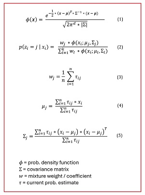 [Click on image for larger view.] Figure 2: The Key Math Equations for GMM Data Clustering
The key symbol in the PDF equation is the Greek uppercase sigma, which represents the covariance matrix. The -1 exponent means the inverse of the matrix. The pair of straight lines means the determinant of the matrix. The inverse and determinant of a covariance matrix are difficult to compute.
Because of the way a covariance matrix is constructed, the most efficient way to compute the inverse and determinant is to use a technique called Cholesky decomposition. Cholesky decomposition is an interesting topic by itself and would take several pages to fully explain. However, it's unlikely that you'll ever have to modify that part of the demo code, so you can consider the inverse and determinant functions as black boxes. See my article "Matrix Inversion Using Cholesky Decomposition With C#" for details.
Computing the Coefficients, Means and Covariance Matrices using EM
Equation (2) in Figure 2 shows how to compute the pseudo-probabilities for a particular data item. The equation corresponds to the worked example presented previously. Fine, but where do the coefficients, means, and covariance matrices come from? The most common meta-algorithm for computing GMM model parameters is called expectation-maximization (EM).
The EM algorithm for GMM data clustering, expressed in very high-level pseudo-code, is:
   loop until very little change in pseudo-probs
      E: use curr coefficients, means, covariances to find probs
      M: use curr probs to update coefficients
         use curr probs to update means
         use curr probs and means to update covariances
    end-loop
    return curr means, covariances, coefficients
In Figure 2, equation (3) shows how to update the coefficients, equation (4) shows how to update the means and equation (5) shows how to update the covariance matrices. If you're a mathematician, you can use the equations to decipher the demo code; if you're a developer, you can use the code to decipher the math equations.
Overall Program Structure
I used Visual Studio 2022 (Community Free Edition) for the demo program. I created a new C# console application and checked the "Place solution and project in the same directory" option. I specified .NET version 6.0. I named the project GaussianMixture. I checked the "Do not use top-level statements" option to avoid the program entry point shortcut syntax.
The demo has no significant .NET dependencies and any relatively recent version of Visual Studio with .NET (Core) or the older .NET Framework will work fine. You can also use the Visual Studio Code program if you like.
After the template code loaded into the editor, I right-clicked on file Program.cs in the Solution Explorer window and renamed the file to the slightly more descriptive GaussianMixtureProgram.cs. I allowed Visual Studio to automatically rename class Program.
The overall program structure is presented in Listing 1. The GaussianMixtureProgram class houses the Main() method, which has all the control logic, and has functions to load data from a text file into memory. The GMM class houses all the Gaussian mixture model clustering functionality. You can see there are a lot of helper methods and functions. All the helpers are relatively simple so the GMM class complexity is due mostly to the interactions and dependencies between the helpers.
Listing 1:
Overall Program Structure
using System;
using System.IO;

namespace GaussianMixture
{
  internal class GaussianMixtureProgram
  {
    static void Main(string[] args)
    {
      Console.WriteLine("Begin GMM from scratch C# ");

      // 1. load data into memory
      // 2. instantiate a GMM object
      // 3. use GMM object to cluster the data
      // 4. display clustering results

      Console.WriteLine("End demo ");
      Console.ReadLine();
    } // Main

    static double[][] MatCreate(int rows, int cols) { . . }

    static int NumNonCommentLines(string fn,
      string comment) { . . }

    static double[][] MatLoad(string fn, int[] usecols,
      char sep, string comment) { . . }

    static void MatShow(double[][] m, int dec, int wid) { . . }

    static void VecShow(double[] vec, int dec, int wid,
      bool newLine) { . . }

  } // Program

  public class GMM
  {
    // ------------------------------------------------------

    public int k;  // number clusters
    public int maxIter;
    public Random rnd;  // for initialization
    public int N;  // number data items
    public int dim;  // per data item

    public double[] coefs;
    public double[][] means;  // init'ed by Cluster()
    public double[][][] covars;  // init'ed by Cluster()
    public double[][] probs; // computed clustering probs

    // ------------------------------------------------------

    public GMM(int k, int maxIter, int seed) { . . }

    public int Cluster(double[][] X) { . . }

    public double[] PredictProbs(double[] x) { . . }

    public double[][] PredictProbs(double[][] X) { . . }

    public int[] PredictLabels(double[][] X) { . . }

    private static int ArgMax(double[] vec) { . . }

    private void ExpectStep(double[][] X) { . . }

    private void MaximStep(double[][] X) { . . }

    public double MeanLogLikelihood() { . . }

    static double[][] LocalVecVecScale(double[] x,
      double[] u, double scale) { . . }

    private int[] Select(int N, int n) { . . }

    private void Shuffle(int[] indices) { . . }

    static double LocalMatGaussianPdf(double[] x,
      double[] u, double[][] covar) { . . }

    static double[][] LocalVecToMat(double[] vec,
      int nRows, int nCols) { . . }

    static double[][] LocalMatTranspose(double[][] m) { . . }

    static double[][] LocalMatDiff(double[][] A,
      double[][] B) { . . }

    static double[][] LocalMatProduct(double[][] matA,
      double[][] matB) { . . }

    static double[][] LocalMatCholesky(double[][] m) { . . }

    static double[][]
      LocalMatInverseFromCholesky(double[][] L) { . . }

    static double
      LocalMatDeterminantFromCholesky(double[][] L) { . . }

    static double[][] LocalMatIdentity(int n) { . . }

    static double[][] LocalMatCreate(int rows,
      int cols) { . . }

    static double[][][] LocalMat3DCreate(int factors,
      int rows, int cols) { . . }

    static void LocalMatShow(double[][] m, int dec,
      int wid) { . . }

    static void LocalVecShow(double[] vec, int dec,
      int wid) { . . }

  } // class GMM
} // ns