The Data Science Lab
Multi-Class Classification Using LightGBM
Dr. James McCaffrey of Microsoft Research provides a full-code, step-by-step machine learning tutorial on how to use the LightGBM system to perform multi-class classification using Python and the scikit-learn library.
A multi-class classification problem is one where the goal is to predict a discrete variable that has three or more possible values. For example, you might want to predict a person's political leaning (conservative, moderate, liberal) from sex, age, state of residence and annual income. There are many machine learning techniques for multi-class classification. One of the most powerful techniques is to use the LightGBM (lightweight gradient boosting machine) system.
LightGBM is a sophisticated, open-source, tree-based system that was introduced in 2017. LightGBM can perform multi-class classification, binary classification (predict one of two possible values), regression (predict a single numeric value) and ranking.
The best way to see where this article is headed is to take a look at the screenshot of a demo program in Figure 1. LightGBM has three programming language interfaces -- C, Python and R. The demo program uses the Python language API. The demo begins by loading the data to analyze into memory. The data looks like:
[1.  24.  0.  29500.]  | 2
[0.  39.  2.  51200.]  | 1
[1.  63.  1.  75800.]  | 0
. . .
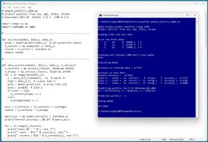 [Click on image for larger view.] Figure 1: LightGBM Multi-Class Classification in Action.
There are 200 items in the training dataset and 40 items in a test dataset. Each line represents a person. The predictor variables are sex, age, state and income. The target class label to predict is political leaning (0 = conservative, 1 = moderate, 2 = liberal).
The demo creates and trains a LightGBM classifier object. The trained model predicts the training data with 97.5 percent accuracy (195 out of 200 correct) and the test data with 82.5 percent accuracy (33 out of 40 correct).
The demo concludes by predicting political leaning for a new, previously unseen person who is male, age 35, from Oklahoma, who make $55,000 a year. The prediction is 2 = liberal.
This article assumes you have intermediate or better programming skill with a C-family language and a basic knowledge of decision tree terminology but does not assume you know anything about LightGBM. The entire source code for the demo program is presented in this article and is also available in the accompanying file download. You can also find the source code and data here.
The Data
The demo program uses a 240-item set of synthetic data. The raw data looks like:
F  24  michigan  29500.00  liberal
M  39  oklahoma  51200.00  moderate
F  63  nebraska  75800.00  conservative
M  36  michigan  44500.00  moderate
F  27  nebraska  28600.00  liberal
. . .
The fields are sex (M, F), age, state (Michigan, Nebraska, Oklahoma), income and political leaning (conservative, moderate, liberal). When using LightGBM, it's best to encode categorical predictors and labels using zero-based ordinal encoding. Unlike most other multi-class classification systems, when using LightGBM, numeric predictor variables can be used as-is. You can normalize numeric predictors using min-max, z-score, or divide-by-constant normalization, but normalization does not help LightGBM models.
You can encode your data in a preprocessing step, or you can encode programmatically while the data is being loaded into memory. The demo uses preprocessing. The comma-delimited encoded data looks like:
1, 24, 0, 29500.00, 2
0, 39, 2, 51200.00, 1
1, 63, 1, 75800.00, 0
0, 36, 0, 44500.00, 1
1, 27, 1, 28600.00, 2
. . .
The 240-item encoded data was split into a 200-item set of training data to create a prediction model and a 40-item set of test data to evaluate the model.
Installing Python and LightGBM
To use the Python language API for LightGBM, you must have Python installed on your machine. I strongly recommend using the Anaconda distribution of Python. The Anaconda distribution contains a Python interpreter and roughly 500 Python packages that are compatible with one another. The demo uses version Anaconda3-2023.09-0, which contains Python version 3.11.5. To install Anaconda on a Windows platform, go here and find installer file Anaconda3-2023.09-0-Windows-x86_64.exe (or newer). Note: it is all-too-easy to download a version that's not compatible with your machine.
Click on the .exe file link to download it to your machine. After the file is on your machine, double-click on the file to start the GUI-based installation process. In most scenarios, you can accept all the default installation values except the one which does not add Anaconda3 to your machine's PATH environment variable -- I recommend adding it so that you don't have to manually edit your system environment variables, or enter long paths on the command line.
You can also follow detailed step-by-step instructions for installing Anaconda Python.
You can verify your Anaconda Python installation by opening a command shell and typing the command "python" (without quotes). You should see a reply message that indicates the version of Python, followed by the Python triple greater-than prompt. You can type "exit()" to quit the interpreter.
If you ever need to uninstall Anaconda on a Windows machine, you can do so by going to the Add or Remove Programs setting and clicking on the Uninstall option.
At the time this article was written, the Anaconda distribution does not contain the LightGBM system, and so it must be installed separately. I strongly recommend using the pip installer program (which is included with Anaconda). To install the most recent version of LightGBM over the internet, open a command shell and type the command "pip install lightgbm." After a few seconds, you should see a message indicating success. To verify, open a command shell and type "python." At the Python prompt, type the command "import lightgbm as L" followed by the command "L.__version__" using double underscores. You should see the version of LightGBM that is installed.
Instead of installing LightGBM over the internet, you can first download the LigbtGBM package to your machine and then install. Go here and search for "lightgbm." The search results will give you a link to a LightGBM package page. Click on the Download Files link. You will go to a page that has a .whl file named like lightgbm-4.3.0-py3-none-win_amd64.whl that you can click on to download the file to your machine. After the download completes, open a command shell, navigate to the directory containing the .whl file and install LightGBM by typing the command "pip install [the .whl file name]."
If you ever need to uninstall LightGBM, you can do so by typing the command "pip uninstall lightgbm." I often use the local-install technique so that I can have a copy of LightGBM on my machine.
The LightGBM Demo Program
The complete demo program is presented in Listing 1. The demo begins by loading the training data into memory:
import numpy as np
import lightgbm as lgbm

def main():
  # 0. get started
  np.random.seed(1)

  # 1. load data
  train_file = ".\\Data\\people_train.txt"
  train_x = np.loadtxt(train_file, usecols=[0,1,2,3],
    delimiter=",", comments="#", dtype=np.float64)
  train_y = np.loadtxt(train_file, usecols=4,
    delimiter=",", comments="#", dtype=np.int64)
. . .
The demo does not use the NumPy random number generator directly, but it's good practice to set the generator seed value anyway in case the program is modified to use the RNG.
The demo assumes that the training and test data files are located in a subdirectory named Data. The comma-delimited data is loaded into NumPy arrays using the loadtxt() function. The predictor values in columns 0, 1, 2, 3 are loaded as type float64 and the labels are loaded as type int64. Lines that begin with "#" are comments and are not loaded.
Listing 1: LightGBM Multi-Class Demo Program
# people_politics_lgbm.py
# predict politics from sex, age, State, income
# Anaconda3-2023.09-0  Python 3.11.5  LightGBM 4.3.0

import numpy as np
import lightgbm as lgbm

# -----------------------------------------------------------

def accuracy(model, data_x, data_y):
  # simple
  preds = model.predict(data_x)  # all predicted values
  n_correct = np.sum(preds == data_y)
  result = n_correct / len(data_x)
  return result

# -----------------------------------------------------------

def show_accuracy(model, data_x, data_y, n_classes):
  # more details
  n_corrects = np.zeros(n_classes, dtype=np.int64)
  n_wrongs = np.zeros(n_classes, dtype=np.int64)
  for i in range(len(data_x)):
    x = data_x[i].reshape(1, -1)  # batch it
    trgt = data_y[i]  # scalar like 2
    pred = model.predict(x)  # array like [2]
    pred = pred[0]  # like 2
    if pred == trgt:
      n_corrects[trgt] += 1
    else:
      n_wrongs[trgt] += 1

  accs = n_corrects / (n_corrects + n_wrongs)
  counts = n_corrects + n_wrongs

  macro_acc = np.sum(n_corrects) / len(data_x)
  print("Overall accuracy = %8.4f" % macro_acc)

  for c in range(n_classes):
    print("class %d : " % c, end ="")
    print(" ct = %3d " % counts[c], end="")
    print(" correct = %3d " % n_corrects[c], end ="")
    print(" wrong = %3d " % n_wrongs[c], end ="")
    print(" acc = %7.4f " % accs[c])

# -----------------------------------------------------------

def confusion_matrix_multi(model, data_x, data_y, n_classes):
  # assumes n_classes is 3 or greater ")
  cm = np.zeros((n_classes,n_classes), dtype=np.int64)
  for i in range(len(data_x)):
    x = data_x[i].reshape(1, -1)  # batch it
    trgt_y = data_y[i]  # scalar like 2
    pred_y = model.predict(x)  # array like [2]
    pred_y = pred_y[0]  # like 2
    cm[trgt_y][pred_y] += 1
  return cm

# -----------------------------------------------------------

def show_confusion(cm):
  # cm created using confusion_matrix_multi()
  dim = len(cm)
  mx = np.max(cm)             # largest count in cm
  wid = len(str(mx)) + 1      # width to print
  fmt = "%" + str(wid) + "d"  # like "%3d"
  for i in range(dim):
    print("actual   ", end="")
    print("%3d:" % i, end="")
    for j in range(dim):
      print(fmt % cm[i][j], end="")
    print("")
  print("------------")
  print("predicted    ", end="")
  for j in range(dim):
    print(fmt % j, end="")
  print("")

# -----------------------------------------------------------

def main():
  # 0. get started
  print("\nBegin People predict politics using LightGBM ")
  print("Predict politics from sex, age, State, income ")
  np.random.seed(1)

  # 1. load data that looks like:
  # sex, age, State, income, politics
  # 1, 24, 0, 29500.00, 2
  # 0, 39, 2, 51200.00, 1
  # . . .
  print("\nLoading train and test data ")
  train_file = ".\\Data\\people_train.txt"
  train_x = np.loadtxt(train_file, usecols=[0,1,2,3],
    delimiter=",", comments="#", dtype=np.float64)
  train_y = np.loadtxt(train_file, usecols=4,
    delimiter=",", comments="#", dtype=np.int64)

  test_file = ".\\Data\\people_test.txt"
  test_x = np.loadtxt(test_file, usecols=[0,1,2,3],
    delimiter=",", comments="#", dtype=np.float64)
  test_y = np.loadtxt(test_file, usecols=4,
    delimiter=",", comments="#", dtype=np.int64)

  np.set_printoptions(precision=0, suppress=True,
    floatmode='fixed')
  print("\nFirst few train data: ")
  for i in range(3):
    print(train_x[i], end="")
    print("  | " + str(train_y[i]))
  print(". . . ")

  # 2. create and train model
  print("\nCreating and training LGBM multi-class model ")
  params = {
    # 'objective': 'multiclass',  # not needed
    'boosting_type': 'gbdt',  # default
    'num_leaves': 31,  # default
    'max_depth':-1,  # default (unlimited)
    'n_estimators': 50,  # default = 100
    'learning_rate': 0.05,  # default = 0.10
    'min_data_in_leaf': 5,  # default = 20
    'random_state': 0,
    'verbosity': -1  # only fatal. default = 1 error, warn
  }
  model = lgbm.LGBMClassifier(**params)  # scikit API
  model.fit(train_x, train_y)
  print("Done ")

  # 3. evaluate model
  print("\nEvaluating model ")

  # 3a. using a coarse function
  train_acc = accuracy(model, train_x, train_y)
  print("\nAccuracy on training data = %0.4f " % train_acc)
  test_acc = accuracy(model, test_x, test_y)
  print("Accuracy on test data = %0.4f " % test_acc)

  # 3b. using a detailed function
  print("\nAccuracy on test data: ")
  show_accuracy(model, test_x, test_y, n_classes=3)

  # 3c. using a confusion matrix
  print("\nConfusion matrix for test data: ")
  cm = confusion_matrix_multi(model, test_x,
    test_y, n_classes=3)
  show_confusion(cm)

  # 4. use model
  print("\nPredicting politics for M 35 Oklahoma $55,000 ")
  print("(0 = conservative, 1 = moderate, 2 = liberal) ")
  x = np.array([[0, 35, 2, 55000.00]], dtype=np.float64)
  pred = model.predict(x)
  print("\nPredicted politics = " + str(pred[0]))

  # 5. save model
  import pickle
  print("\nSaving model ")
  pth = ".\\Models\\politics_model.pkl"
  with open(pth, "wb") as f:
    pickle.dump(model, f)

  # with open(pth, "rb") as f:
  #   model2 = pickle.load(f)
  #
  # x = np.array([[0, 35, 2, 55000.00]], dtype=np.float64)
  # pred = model2.predict(x)
  # print("\nPredicted politics = " + str(pred[0]))

  print("\nEnd demo ")

if __name__ == "__main__":
  main()
The test data is loaded into memory as arrays test_x and test_y in the same way as the training data. Next, the demo displays the first three lines of the training data as a sanity check:
  np.set_printoptions(precision=0, suppress=True,
    floatmode='fixed')
  print("First few train data: ")
  for i in range(3):
    print(train_x[i], end="")
    print("  | " + str(train_y[i]))
  print(". . . ")
In a non-demo scenario, you might want to display all the data.