The Data Science Lab
How to Do Kernel Logistic Regression Using C#
Dr. James McCaffrey of Microsoft Research uses code samples, a full C# program and screenshots to detail the ins and outs of kernal logistic regression, a machine learning technique that extends regular logistic regression -- used for binary classification -- to deal with data that is not linearly separable.
Regular logistic regression is a machine learning technique that can be used for binary classification. An example is predicting whether a person is male or female based on predictor variables such as age, height, weight, and so on. One weakness of regular logistic regression is that the technique doesn't work well with data that is not linearly separable. Kernel logistic regression is a technique that extends regular logistic regression to deal with data that is not linearly separable.
A good way to understand what kernel logistic regression is and to see where this article is headed is to examine the screenshot of a demo program in Figure 1 and a graph of the associated data in Figure 2. The goal of the demo is to predict whether a data item is class 0 or class 1 based on two predictor variables. The demo uses just two predictors so that the data can be visualized in a graph, but kernel logistic regression can handle any number of predictors. You can imagine that the demo corresponds to a problem where you want to predict if a person is male (class 0, red) or female (class 1, blue) based on age (predictor x0) and weight (predictor x1).
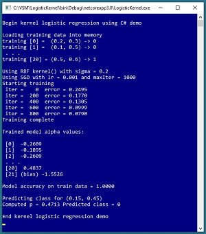 [Click on image for larger view.] Figure 1: Kernel Logistic Regression in Action
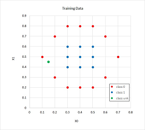 [Click on image for larger view.] Figure 2: The Training/Reference Data
Linearly separable data is data where it is possible to split the two classes by drawing a straight line (or by a hyperplane when there are three or more predictor variables). The demo data is far from being linearly separable and regular logistic regression would give you a model with only about 57 percent accuracy -- not much better than randomly guessing the class. Notice that there are 21 data items.
The demo program begins by loading the training data into memory. Kernel logistic regression requires you to specify a kernel function and parameters for the kernel function. The demo uses a radial basis function (RBF) kernel function. The RBF function has a single parameter, sigma, which is set to 0.2 by the demo. The choice of which kernel function to use and the values of the function's parameters are meta hyperparameters that must be determined using trial and error.
Behind the scenes, the demo program uses stochastic gradient descent to train the kernel logistic regression model. Training is an iterative process. The demo sets the number of training iterations to 1,000 and the learning rate, which controls how much the model's parameters change on each update, to 0.001. The number of training iterations and the learning rate are hyperparameters.
After training completed, the demo displayed a few of the values of the model's 21 alpha values and the one bias value. A kernel logistic regression model will have one alpha value for each training item, and one bias value.
The resulting model has 100 percent accuracy -- predicting the class of all 21 training items correctly. The demo concludes by making a prediction for a new, previously unseen data item with predictor values (0.15, 0.45). The model output is p = 0.4713 and because that value is less than 0.5 the predicted class is class 0.
This article assumes you have intermediate or better skill with C# but doesn’t assume you know anything about kernel logistic regression binary classification. The code for demo program is a bit too long to present in its entirety in this article but the complete code is available in the associated file download.
Understanding the Radial Basis Function
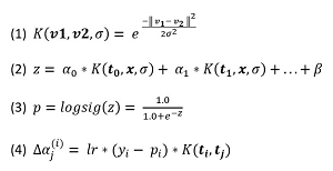
The most common kernel function used by kernel logistic regression, and the one used in the demo program, is the radial basis function (RBF). The RBF definition, expressed in math terms, is shown as equation (1) in Figure 3. The function accepts two vectors, v1 and v2, and a sigma value. The double-bar notation is the norm/length of a vector, which is the square root of the sum of the squared components of the vector. For example, if v = (1.0, 4.0, 2.0) then || v || = sqrt( 1.0^2 + 4.0^2 + 2.0^2 ) = sqrt(1.0 + 16.0 + 4.0) = sqrt(21.0) = 4.58.
 [Click on image for larger view.] Figure 3: Equations for Kernel Logistic Regression
Notice that equation (1) squares the norm, which undoes the square root operation. Because of this, || v || is sometimes called the squared length of vector v.
Suppose v1 = (4, 7, 3) and v2 = (1, 6, 5) and sigma = 1.5. The vector difference is v1 -- v2 = (4-1, 7-6, 3-5) = (3, 1, -2). The squared length of the difference is 3^2 + 1^2 + (-2)^2 = 9 +1 + 4 = 14.0. The denominator is 2 * sigma^2 = 2 * (1.5)^2 = 2 * 2.25 = 4.5. The final value of the kernel function is exp(-14.0 / 4.5) = exp(-3.1111) = 0.0446.
The demo program implements the RBF function like so:
static double Kernel(double[] v1, double[] v2,
  double sigma)
{
  double num = 0.0;
  for (int i = 0; i < v1.Length; ++i)
    num += (v1[i] - v2[i]) * (v1[i] - v2[i]);
  double denom = 2.0 * sigma * sigma;
  double z = num / denom;
  return Math.Exp(-z);
}
The function could be tested using these statements:
double[] v1 = new double[] { 4, 7, 3 };
double[] v2 = new double[] { 1, 6, 5 };
double x = Kernel(v1, v2, 1.5);
Console.WriteLine(x);  // 0.0446
One way to think about the RBF function is that it's a metric that describes the similarity of two vectors. If the two vectors have the same values, RBF returns 1.0 (maximum similarity). For example, if v1 = (2, 6, 4) and v2 = (2, 6, 4) then RBF is 1.0. The more different the two vectors are, the smaller the value of RBF is, approaching but never quite reaching 0.0 (minimum similarity).
Understanding Kernel Logistic Regression
The input-output mechanism for kernel logistic regression, expressed mathematically, is shown as equations (2) and (3) in Figure 3. The mechanism is a bit tricky and is perhaps best explained by a concrete example. Suppose you have just four training items and each training item has just two predictor variables:
[0]  0.2  0.6
[1]  0.3  0.4
[2]  0.1  0.9
[3]  0.5  0.7
A trained kernel logistic regression model will have four alpha values and one bias value. Suppose the alpha values are (1.0, -1.2, 1.3, 1.4) and the bias (sometimes called the beta value) is -2.0 and you set sigma to 0.25. Now suppose you want to make a prediction for an input of (0.8, 0.2). The calculations are:
z = 1.0 * K( (0.2, 0.6), (0.8, 0.2), 0.25 ) +
   -1.2 * K( (0.3, 0.4), (0.8, 0.2), 0.25 ) +
    1.3 * K( (0.1, 0.9), (0.8, 0.2), 0.25 ) +
    1.4 * K( (0.5, 0.7), (0.8, 0.2), 0.25 ) + (-2.0)

  = 1.0 * 0.0156 +
   -1.2 * 0.0983 +
    1.3 * 0.0004 +
    1.4 * 0.0659 + (-2.0)

  = -2.0096

p = logsig(-2.0096) = 1.0 / (1.0 + exp(+2.0096))
  = 0.1182
In words, to compute the output for an input vector, you compute the similarity metric of the input vector with each of the training items, weighting each similarity term by an associated alpha value, then add the bias value, and then apply the logistic sigmoid function. The resulting p-value will be between 0.0 and 1.0 and if the p-value is less than 0.5 the prediction is class 0, otherwise the prediction is class 1.
OK, but where do the alpha values and the beta/bias value come from? These values must be determined by training the model using data with known correct input and output values. The alphas and bias are initially set to 0.0 and then iteratively adjusted by a small amount so that the computed output p-value is closer to the target 0 or 1 correct value.
Notice that after training a kernel logistic regression binary classification model, you still need the training data to make a prediction. This is different from techniques like regular logistic regression or neural network models where the training data is not needed after the model has been created. For this reason, in a kernel logistic regression context, the training data is sometimes called reference data.
Training a Kernel Logistic Regression Model
There are several techniques that can be used to find good values for kernel logistic regression alphas and the bias. The demo program uses a simplified form of stochastic gradient descent (SGD). The update delta value for the alpha associated with training item [j] and associated input vector [i] is shown as equation (4) in Figure 3. In the equation, y(i) is the target output value (0 or 1) for input [i] and p(i) is the computed p-value (between 0.0 and 1.0).
Suppose, for a given set of alphas and bias, the computed output p(i) is 0.7 and the target value is y(i) = 1. The computed output gives a correct prediction but you'd like p(i) to be somewhat greater so that it's closer to the target value. The difference y(i) -- p(i) is 1 -- 0.7 = +0.3 so you could add this delta to the current value of alpha and p(i) would increase. However, this update strategy is too aggressive so you throttle the delta using two terms. The learning rate, a value typically something like 0.01 or 0.05, will reduce the delta value. And the value of the kernel function will adjust the delta value so that training items that are close to the input vector will get more weight than training items that are dissimilar to the input vector.
To update the single bias value, you can use equation (4) in Figure 3 and use a dummy value of 1.0 in place of the value of the kernel function. The form of SGD used in the demo program is simple and relatively crude compared to other forms of SGD. In particular, the update equation uses the Calculus derivative of the error term but does not use the derivative of the logistic sigmoid function, which is p(i) * (1 - p(i)). However, the simple approach usually works well in practice.
The Demo Program
To create the demo program, I launched Visual Studio 2019. I used the Community (free) edition but any relatively recent version of Visual Studio will work fine. From the main Visual Studio start window I selected the "Create a new project" option. Next, I selected C# from the Language dropdown control and Console from the Project Type dropdown, and then picked the "Console App (.NET Core)" item.
The code presented in this article will run as a .NET Core console application or as a .NET Framework application. Many of the newer Microsoft technologies, such as the ML.NET code library, specifically target .NET Core so it makes sense to develop most new C# machine learning code in that environment.
I entered "LogisticKernel" as the Project Name, specified C:\VSM on my local machine as the Location (you can use any convenient directory), and checked the "Place solution and project in the same directory" box.
After the template code loaded into Visual Studio, at the top of the editor window I removed all using statements to unneeded namespaces, leaving just the reference to the top-level System namespace. The demo needs no other assemblies and uses no external code libraries.
In the Solution Explorer window, I renamed file Program.cs to the more descriptive LogisticKernelProgram.cs and then in the editor window I renamed class Program to class LogisticKernelProgram to match the file name. The structure of the demo program, with a few minor edits to save space, is shown in Listing 1.
Listing 1. Kernel Logistic Regression Demo Program Structure
using System;
namespace LogisticKernel
{
  class LogisticKernelProgram
  {
    static void Main(string[] args)
    {
      Console.WriteLine("Begin kernel LR demo ");
      Console.WriteLine("Loading training data");
      Console.WriteLine("train [0] =  (0.2, 0.3) 0");
      Console.WriteLine("train [1] =  (0.1, 0.5) 0");
      Console.WriteLine(" . . . ");
      Console.WriteLine("train [20] = (0.5, 0.6) 1");

      double[][] trainX = new double[21][];
      trainX[0] = new double[] { 0.2, 0.3 };
      trainX[1] = new double[] { 0.1, 0.5 };
      . . .
      trainX[19] = new double[] { 0.5, 0.5 };
      trainX[20] = new double[] { 0.5, 0.6 };

      int[] trainY = new int[21] {
        0, 0, 0, 0, 0, 0, 0, 0, 0, 0, 0, 0,
        1, 1, 1, 1, 1, 1, 1, 1, 1 };

      int maxIter = 1000;
      double lr = 0.001;
      double sigma = 0.2;

      Console.WriteLine("sigma = " + sigma);
      Console.WriteLine("lr = " + lr +
        " and maxIter = " + maxIter);
      Console.WriteLine("Starting training");
      double[] alphas = Train(trainX, trainY,
        lr, maxIter, sigma);
      Console.WriteLine("Training complete");

      ShowSomeAlphas(alphas, 3, 2);

      double accTrain = Accuracy(trainX, trainY,
        trainX, alphas, sigma);
      Console.WriteLine("accuracy = " +
        accTrain.ToString("F4") + "\n");

      Console.WriteLine("Predicting (0.15, 0.45)");
      double[] unknown = new double[] { 0.15, 0.45 };
      double p = ComputeOutput(unknown, alphas,
        sigma, trainX);
      if (p < 0.5)
        Console.WriteLine("Computed p = " +
          p.ToString("F4") +
          " Predicted class = 0");
      else
        Console.WriteLine("Computed p = " +
          p.ToString("F4") +
          " Predicted class = 1");

      Console.WriteLine("End kernel LR demo ");
      Console.ReadLine();

    } // Main

    static double[] Train(double[][] trainX,
      int[] trainY, double lr, int maxIter,
      double sigma, int seed = 0) { . . }

    static double Kernel(double[] v1, double[] v2,
      double sigma) { . . }

    static double ComputeOutput(double[] x,
      double[] alphas, double sigma,
      double[][] trainX) { . . }

    static double LogSig(double x) { . . }

    static double Error(double[][] dataX,
      int[] dataY, double[][] trainX,
      double[] alphas, double sigma) { . . }

    static double Accuracy(double[][] dataX,
      int[] dataY, double[][] trainX,
      double[] alphas, double sigma) { . . }

    static void Shuffle(int[] indices,
      Random rnd) { . . }

    static void ShowSomeAlphas(double[] alphas,
      int first, int last) { . . }

  } // Program class
} // ns