The Data Science Lab

How to Do Multi-Class Logistic Regression Using C#

Dr. James McCaffrey of Microsoft Research uses a full code program, examples and graphics to explain multi-class logistic regression, an extension technique that allows you to predict a class that can be one of three or more possible values, such as predicting the political leaning of a person (conservative, moderate, liberal) based on age, sex, annual income and so on.

• By James McCaffrey
• 02/11/2020

Basic logistic regression classification is arguably the most fundamental machine learning (ML) technique. Basic logistic regression can be used for binary classification, for example predicting if a person is male or female based on predictors such as age, height, annual income, and so on. Multi-class logistic regression is an extension technique that allows you to predict a class that can be one of three or more possible values. An example of multi-class classification is predicting the political leaning of a person (conservative, moderate, liberal) based on age, sex, annual income and so on.

Many machine learning code libraries have built-in multi-class logistic regression functionality. However, coding multi-class logistic regression from scratch has least four advantages over using a library. Your code can be small and efficient, you can avoid licensing and copyright issues, you have full ability to customize your system, and it's usually easier to integrate your multi-class logistic regression code into other systems.

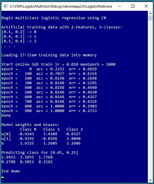
A good way to get a feel for what multi-class logistic regression classification is and to see where this article is headed is to take a look at the screenshot of a demo program in Figure 1. The goal of the demo is to create a model that predicts if a data item is one of three classes, class 0, class 1, or class 2, based on two predictor values, x0 and x1.

To keep the main ideas of multi-class logistic regression as clear as possible, the demo program uses synthetic data with 27 items. The demo uses stochastic gradient descent for 1,000 epochs (iterations) and a learning rate set to 0.010 to train the model.

During training, the accuracy of the model slowly improves from 0.3333 accuracy (9 of 27 correct) with a mean squared error of 0.6659, to 1.0000 accuracy (27 of 27 correct) with 0.3713 mean squared error.

After training, the model is used to predict the class of a new, previously unseen data item with predictor values x0 = 0.45 and x1 = 0.25. The raw prediction output is (1.9913, 2.5855, 1.7368) which correspond to classes 0, 1, 2 respectively. Because the value at [1] is largest, the prediction is class 1.

The demo also displays predicted output in a softmax-normalized form of (0.2788, 0.5051, 0.2162) where the prediction values sum to 1.0 and can loosely be interpreted as probabilities. Therefore, the prediction is that the item is class 1 with a 0.5051 pseudo-probability.

This article assumes you have intermediate or better skill with C# but doesn't assume you know anything about multi-class logistic regression classification. The code for demo program is a bit too long to present in its entirety in this article but the complete code is available in the associated file download.

Understanding the Data
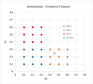
The demo program uses a small 27-item dataset that was artificially generated. The data is shown in the graph in Figure 2. There are only two predictor variables (often called features in ML terminology) so that the data can be displayed in a two-dimensional graph. Most real-life training data will have more than two predictors.

For concreteness you can image that the synthetic training data corresponds to a problem where the goal is to predict the political leaning of a person (conservative = class 0, moderate = class 1, liberal = class 2) based on x0 = age and x1 = annual income.

Both basic logistic regression and multi-class logistic regression only work well with data that is nearly linearly separable. For two-dimensional data this means it's possible to draw straight lines that separate the data into distinct classes. For higher dimensional data this means that it's possible to separate the data using hyperplanes. The graph in Figure 2 shows that the synthetic training data is fully linearly separable, which rarely happens with real-world data.

The graph in Figure 2 displays the unknown item predicted by the demo program at (0.45, 0.25) as a green circle. Visual inspection indicates that the unknown item should be classified as class 1, but with small likelihoods of being class 0 or class 2. This intuition corresponds to the pseudo-probability output values of (0.2788, 0.5051, 0.2162).

Understanding How Multi-Class Logistic Regression Classification Works
Multi-class logistic regression is based on regular binary logistic regression. For regular logistic regression, if you have a dataset with n predictor variables, there will be n weights plus one special weight called a bias. Weights and biases are just numeric constants with values like -1.2345 and 0.9876.

To make a prediction, you sum the products of each predictor value and its associated weight and then add the bias. The sum is often given the symbol z. Then you apply the logistic sigmoid to z to get a p-value. If the p-value is less than 0.5 then the prediction is class 0 and if the p-value is greater than or equal to 0.5 then the prediction is class 1.

For example, suppose you have a dataset with three predictor variables with values (5.0, 6.0, 7.0) and suppose that the three associated weight values are (0.20, -0.40, 0.30) and the bias value is 1.10. Then:

z = (0.20 * 5.0) + (-0.40 * 6.0) + (0.30 * 7.0) + 1.10 
   = 1.80
p = 1.0 / (1.0 + exp(-1.80))
   = 0.8581

Because p is greater than or equal to 0.5 the predicted class is 1.

The function f(x) = 1.0 / (1.0 + exp(-x)) is called the logistic sigmoid function (sometimes called just the sigmoid function when the context is clear). The function exp(x) is Euler's number, approximately 2.718, raised to the power of x. If y = exp(x) the Calculus derivative is y * (1 – y) which turns out to be important when training a basic logistic regression model

Multi-class logistic regression is perhaps best explained using an example. Suppose, as in the demo program, your dataset has two predictor variables and there are three possible classes.

Instead of one z value, you will have three z values, one for each class. And instead of applying the logistic sigmoid function to one z value which gives a single value between 0.0 and 1.0, you apply the softmax function to the three z values which results in a vector with three p values which sum to 1.0.

Suppose the item to predict is x0 = 1.0 and x2 = 2.0. For each of the three z values you need two weights and one bias. Suppose the weights and bias for z0 are (0.1, 0.2, 0.3), the weights and bias for z1 are (04, 0.5, 0.6), and the weights and bias for z2 are (0.7, 0.8, 0.9). The three z values are computed as:

z0 = (0.1 * 1.0) + (0.2 * 2.0) + 0.3 = 0.80
z1 = (0.4 * 1.0) + (0.5 * 2.0) + 0.6 = 2.00
z2 = (0.7 * 1.0) + (0.8 * 2.0) + 0.9 = 3.20

The three probabilities are computed as the softmax(z0, z1, z2):

p0 = exp(0.80) / [exp(0.80) + exp(2.00) + exp(3.20)]
     = 2.23 / 34.15
     = 0.0652

p1 = exp(2.00) / [exp(0.80) + exp(2.00) + exp(3.20)]
     = 7.39 / 34.15
     = 0.2164

p2 = exp(3.20) / [exp(0.80) + exp(2.00) + exp(3.20)]
     = 24.53 / 34.15
     = 0.7184

In words, the softmax of a set of values is the exp() of each value divided by the sum of the exp() of all values. In this example, because the p2 pseudo-probability is the largest, the prediction is class 2.

Although it's not obvious, there is a very close but complex mathematical relationship between the logistic sigmoid function used for basic logistic regression, and the softmax function used for multi-class logistic regression.

Error and Accuracy
Computing output values for multi-class logistic regression is not difficult but where do the values of the weights and biases come from? The process of determining the values of the weights and biases is called training the model. The idea is to use a set of training data that has known input values and known, correct output values to find values for the weights and biases so that the error between computed output values and the known correct values is minimized.

Suppose you have a problem where there are three possible classes. In the training data you encode correct output values (sometimes called the target values) using the one-hot scheme where class 0 is encoded as (1, 0, 0), class 1 is encoded as (0, 1, 0), and class 2 is encoded as (0, 0, 1). A computed output will have three values between 0.0 and 1.0 that can be considered pseudo-probabilities.

Suppose an item of training data has a correct class of 2 encoded as (0, 0, 1) and suppose that the associated computed output using a set of weights and biases is (0.20, 0.10, 0.70). The squared error for this one training item is (0 – 0.20)^2 + (0 – 0.10)^2 + (1 – 0.70)^2 = 0.04 + 0.01 + 0.09 = 0.14.

If you have N training data items, the mean squared error (MSE) for the set is one-half of the sum of the square errors for each training item, divided by N. The one-half factor makes the Calculus derivative of the error function simpler than it would be without the one-half.

An alternative form of error that is sometimes used for multi-class logistic regression is called mean cross entropy error (MCEE). MCEE is often used for neural network classification but MSE is far more common for multi-class logistic regression. The demo program uses MSE.

Error is used during multi-class logistic regression to find good values for the model weights and biases. After training, accuracy tells you how good your model is. Suppose you have three classes with just four training items. Your model gives you these results:

target     predicted
(0, 1, 0)  (0.2, 0.5, 0.3)
(1, 0, 0)  (0.3, 0.4, 0.3)
(0, 0, 1)  (0.1, 0.2, 0.7)
(0, 1, 0)  (0.3, 0.6, 0.1) 

The predicted classes for the first, third and fourth items are correct because the largest pseudo-probability matches the 1 in the target data. But the predicted class for the second item is incorrect because the largest pseudo-probability (0.4) does not match the 1 in the target. Therefore the model has 3 / 4 = 0.75 or 75 percent accuracy.

The Training Algorithm
There are many different algorithms that can be used to train a multi-class logistic regression model and each algorithm has several variations. Common algorithms include stochastic gradient descent (online or batch), L-BFGS, simplex optimization, evolutionary optimization, iterated Newton-Raphson, and stochastic dual coordinate ascent. The demo program uses the online variation of stochastic gradient descent (SGD).

At a high level of abstraction, online SGD is:

loop maxEpoch times
  for-each training item
    compute pseudo-probability outputs
    for-each class and each weight
      update weight so computed is closer to target
    end-for classes and weights
  end-loop items
end-loop epochs

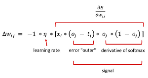
The weight update equation, in math terms, is shown in Figure 3. The delta wij is the value to add to the weight for input i and class j. The learning rate is a small scaling value, often about 0.01 or 0.05, that controls how much each weight is changed. The (oj – tj) term is the difference between the output and the target for class j and is the Calculus derivative of the error function.

The oj * (1 – oj) term is the Calculus derivative of the softmax function. The xi term is the input value associated weight wij. Because bias values do not have an explicit associated input value, the xi term to update a bias value is the constant 1.

The -1 term in the update equation is used so that an update to weight wij is computed by adding the delta value. Some implementations change the (oj – tj) term to (tj – oj) and then drop the -1 term. Another alternative is to drop the -1 term but then subtract the weight delta instead of adding it.

The Demo Program
To create the demo program, I launched Visual Studio 2019. I used the Community (free) edition but any relatively recent version of Visual Studio will work fine. From the main Visual Studio start window I selected the "Create a new project" option. Next, I selected C# from the Language dropdown control and Console from the Project Type dropdown, and then picked the "Console App (.NET Core)" item.

The code presented in this article will run as a .NET Core console application or as a .NET Framework application. Many of the newer Microsoft technologies, such as the ML.NET code library, specifically target .NET Core so it makes sense to develop most new C# M code in that environment.

I entered "LogisticMulti" as the Project Name, specified C:\VSM on my local machine as the Location (you can use any convenient directory), and checked the "Place solution and project in the same directory" box.

After the template code loaded into Visual Studio, at the top of the editor window I removed all using statements to unneeded namespaces, leaving just the reference to the top level System namespace. The demo needs no other assemblies and uses no external code libraries.

• Get Code Download