The Data Science Lab
Logistic Regression Using PyTorch with L-BFGS
Dr. James McCaffrey of Microsoft Research demonstrates applying the L-BFGS optimization algorithm to the ML logistic regression technique for binary classification -- predicting one of two possible discrete values.
Logistic regression is one of many machine learning techniques for binary classification -- predicting one of two possible discrete values. An example is predicting if a hospital patient is male or female based on variables such as age, blood pressure and so on. There are dozens of code libraries and tools that can create a logistic regression prediction model, including Keras, scikit-learn, Weka and PyTorch. When training a logistic regression model, there are many optimization algorithms that can be used, such as stochastic gradient descent (SGD), iterated Newton-Raphson, Nelder-Mead and L-BFGS.
This article explains how to create a logistic regression binary classification model using the PyTorch code library with L-BFGS optimization. A good way to see where this article is headed is to take a look at the screenshot of a demo program in Figure 1.
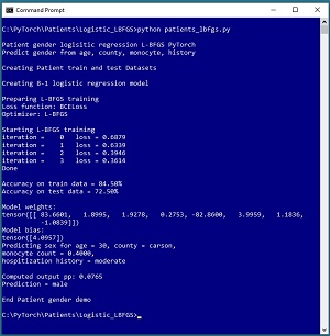 [Click on image for larger view.] Figure 1: Predicting Patient Gender Using Logistic Regression
The goal of the demo is to predict the sex (0 = male, 1 = female) of a hospital patient based on age, county of residence, blood monocyte count and hospitalization history. The demo reads a 200-item set of training data and a 40-item set of test data into memory, then uses the training data to create a logistic regression model using the L-BFGS algorithm.
After training, the demo computes the prediction accuracy of the model on the training data (84.50% = 169 of 200 correct) and the test data (72.50% = 29 of 40 correct). The demo concludes by making a prediction for a new, previously unseen patient data item (age = 30, county = "carson", monocyte = 0.4000, hospitalization history = "moderate"). The computed pseudo-probability output is 0.0765 and because that value is less than 0.5 the prediction is class 0 = male.
This article assumes you have an intermediate or better familiarity with a C-family programming language, preferably Python, and a basic familiarity with the PyTorch code library. The complete source code for the demo program is presented in this article and is also available in the accompanying file download. The training and test data are embedded as comments in the program source file. All normal error checking has been removed to keep the main ideas as clear as possible.
To run the demo program, you must have Python and PyTorch installed on your machine. The demo programs were developed on Windows 10 using the Anaconda 2020.02 64-bit distribution (which contains Python 3.7.6) and PyTorch version 1.8.0 for CPU installed via pip. Installation is not trivial. You can find detailed step-by-step installation instructions in my blog post.
The Patient Dataset
The data used by the demo program is artificial. There is a 200--item dataset for training and a 40-item dataset for testing. The data looks like:
1   0.58   0   1   0   0.6540   0   0   1
0   0.36   1   0   0   0.4450   0   1   0
1   0.55   0   0   1   0.6460   1   0   0
0   0.31   0   1   0   0.4640   1   0   0
. . .
Each tab-delimited line represents a hospital patient. The first column is the variable to predict, gender (0 = male, 1 = female). The other eight columns are the predictor variables: age (normalized by dividing by 100), county of residence (1 0 0 = austin, 0 1 0 = bailey, 0 0 1 = carson), blood monocyte count (a type of white blood cell) and hospitalization history (1 0 0 = minor, 0 1 0 = moderate, 0 0 1 = major).
The demo program defines a PyTorch Dataset class to load training or test data into memory. See Listing 1. Although you can load data from file directly into a NumPy array and then covert to a PyTorch tensor, using a Dataset is the de facto technique used for most PyTorch programs.
Listing 1: A Dataset Class for the Patient Data
import torch as T
import numpy as np

class PatientDataset(T.utils.data.Dataset):
  def __init__(self, src_file, num_rows=None):
    all_data = np.loadtxt(src_file, max_rows=num_rows,
      usecols=range(0,9), delimiter="\t", skiprows=0,
      comments="#", dtype=np.float32)  # read all 9 columns

    self.x_data = T.tensor(all_data[:,1:9],
      dtype=T.float32).to(device)
    self.y_data = T.tensor(all_data[:,0],
      dtype=T.float32).to(device)

    self.y_data = self.y_data.reshape(-1,1)  # 2D

  def __len__(self):
    return len(self.x_data)

  def __getitem__(self, idx):
    preds = self.x_data[idx,:]  # idx rows, all 8 cols
    sex = self.y_data[idx,:]    # idx rows, the only col
    sample = { 'predictors' : preds, 'sex' : sex }
    return sample
The class loads a file of patient data into memory as a two-dimensional array using the NumPy loadtxt() function. The class labels and predictors are separated into two arrays and then converted to PyTorch tensors. Even though the class labels (0 or 1) are conceptually integers, the demo program uses binary cross entropy error which requires a float type.
The Dataset can be called for use by L-BFGS training like this:
fn = ".\\Data\\patient_train.txt "
my_ds = PatientDataset(fn)
my_ldr = T.utils.data.DataLoader(my_ds, \
  batch_size=len(my_ds), shuffle=False)
for (_, batch) in enumerate(my_ldr):
  # _ is the batch index, not used
  # batch has all training items
. . .
When using L-BFGS for training, all data must be passed to the optimizer object. Therefore, the notions of a batch of data and batch training do not apply. This means the DataLoader shuffle parameter can be set to False.
Understanding Logistic Regression
Logistic regression is best explained by example. Suppose that instead of the Patient dataset you have a simpler dataset where the goal is to predict gender from x0 = age, x1 = income and x2 = job tenure. A logistic regression model will have one weight value for each predictor variable, and one bias constant. Suppose that the weights are w0 = 13.5, w1 = -12.2, w2 = 1.08, and the bias is b = 1.12. Now suppose you have a data item where age = x0 = 0.32, income = x1 = 0.62, tenure = x2 = 0.77. The predicted gender is computed as:
z = (x0 * wo) + (x1 * w1) + (x2 * w2) + b
  = (0.32 * 13.5) + (0.62 * -12.2) + (0.77 * 1.08) + 1.12
  = 4.32 + -7.56 + 0.83 + 1.12
  = -1.29

p = 1 / (1 + exp(-z))
  = 1 / (1 + exp(1.29))
  = 1 / (1 + 3.63)
  = 0.22
Because the pseudo-probability value p is less than 0.5, the prediction is class 0 = male.
In words, you compute a z value, which is the sum of weights times inputs, plus the bias. Then you compute a p value which is 1 over 1 plus the exp() applied to -z. The equation for p is called the logistic sigmoid function. When computing logistic regression, a z value can be anything from minus infinity to plus infinity, but a p value will always be between 0 and 1.
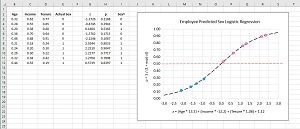 [Click on image for larger view.] Figure 2: Logistic Regression Explained with a Graph
When graphed, the logistic sigmoid function has an "S" shape centered around z = 0. The magnitude of the graph ranges between 0 and 1. Each data item will map to a z value and each z value will map to a point p on the sigmoid function. Values of p that are less than 0.5 lie on the bottom part of the sigmoid curve and correspond to class 0 predictions; values great than 0.5 lie on the top part and correspond to class 1. You can use threshold values other than 0.5 to tune a logistic regression model.
Note that the internet is littered with incorrect graphs of logistic regression where data points are shown both above and below the sigmoid curve. If you ever see a graph like that, you'd be well advised to look for better resources.
OK, this is all good, but where do the values of the weights and bias come from? The process of finding good values for the model weights and bias is called training the model. There is no closed form solution for finding optimal values of the weights and bias and so the values must be estimated using an iterative technique. There are many optimization algorithms for logistic regression training. The demo uses the L-BFGS ("limited memory Broyden Fletcher Goldfarb Shanno") algorithm. The L-BFGS algorithm estimates a Calculus first derivative (gradient) and also a second derivative (Hessian). This requires all data to be in memory but produces very fast training.
Defining the Logistic Regression Model
The class that defines the logistic regression model is:
import torch as T
class LogisticReg(T.nn.Module):
  def __init__(self):
    super(LogisticReg, self).__init__()
    self.fc = T.nn.Linear(8, 1)
    T.nn.init.uniform_(self.fc.weight, -0.01, 0.01)
    T.nn.init.zeros_(self.fc.bias)

  def forward(self, x):
    z = self.fc(x)
    p = T.sigmoid(z)
    return p
The Linear layer computes a sum of weights times inputs, plus the bias. The sigmoid() function applies logistic sigmoid to the sum. The forward() method is called implicitly, for example:
log_reg = LogisticReg().to(device)
X = T.tensor(np.array([0.32, 1,0,0, 0.4567, 0,1,0],
  dtype=np.float32))
pp = log_reg(X)  # not pp = log_reg.forward(X)
The demo uses explicit uniform() initialization for model weights, which often works better than the PyTorch default xavier() initialization algorithm for logistic regression.
Training the Model
The demo program defines a train() function as presented in Listing 2. The train() function defines an LBFGS() optimizer object using default parameter values except for max_iter (maximum iterations). The LBFGS() class has seven parameters which have default values:
lr: default = 1.0
max_iter: default = 20
max_eval: default = max_iter * 1.25
tolerance_grad: default = 1.0e-5
tolerance_change: default = 1.0e-9
history_size: default = 100
line_search_fn: default = None
In most situations the default parameter values work quite well, but you should review the PyTorch documentation to understand what these parameters do so you can modify them if necessary when training fails.
Listing 2: The train() Function
def train(log_reg, ds, mi):
  log_reg.train()
  loss_func = T.nn.BCELoss()  # binary cross entropy
  opt = T.optim.LBFGS(log_reg.parameters(), max_iter=mi)
  train_ldr = T.utils.data.DataLoader(ds,
    batch_size=len(ds), shuffle=False)

  print("Starting L-BFGS training")

  for itr in range(0, mi):
    itr_loss = 0.0            # for one iteration
    for (_, all_data) in enumerate(train_ldr):
      X = all_data['predictors']
      Y = all_data['sex']

      # -------------------------------------------
      def loss_closure():
        opt.zero_grad()
        oupt = log_reg(X)
        loss_val = loss_func(oupt, Y)
        loss_val.backward()
        return loss_val
      # -------------------------------------------

      opt.step(loss_closure)  # get loss, use to update wts

      oupt = log_reg(X)  # monitor loss
      loss_val = loss_closure()
      itr_loss += loss_val.item()
    print("iteration = %4d   loss = %0.4f" % (itr, itr_loss))
  print("Done ")
It's not necessary to explicitly set the model into train() mode because no batch normalization or dropout are used. However, in my opinion it's good practice to set mode even when not technically necessary.
When using L-BFGS optimization, you should use a closure to compute loss (error) during training. A Python closure is a programming mechanism where the closure function is defined inside another function. The closure has access to all the parameters and local variables of the outer container function. This allows the closure function to be passed by name, without parameters, to any statement within the container function. In the case of L-BFGS training, the loss closure computes the loss when the name of the loss function is passed to the optimizer step() method. The technique seems a bit odd if you haven't seen it before but makes sense if you think about it long enough.
Overall Program Structure
The overall demo program structure, with a few minor edits to save pace, is presented in Listing 3. The demo begins by importing the required core NumPy and Torch libraries. It's a good idea to document the versions of libraries being used because PyTorch is under continuous development.
Listing 3:
Overall Logistic Regression Program Structure
# patients_lbfgs.py
# Logistic Regression using PyTorch with L-BFGS optimization
# predict sex from age, county, monocyte, history
# PyTorch 1.8.0-CPU Anaconda3-2020.02  Python 3.7.6
# Windows 10

import numpy as np
import torch as T
device = T.device("cpu")

# ----------------------------------------------------------

class PatientDataset(T.utils.data.Dataset):
  # see Listing 1

class LogisticReg(T.nn.Module):
  def __init__(self):
    super(LogisticReg, self).__init__()
    self.fc = T.nn.Linear(8, 1)
    T.nn.init.uniform_(self.fc.weight, -0.01, 0.01)
    T.nn.init.zeros_(self.fc.bias)

  def forward(self, x):
    z = self.fc(x)
    p = T.sigmoid(z)
    return p

def train(log_reg, ds, mi):
  # see Listing 2

def accuracy(model, ds, verbose=False):
  # see Listing 4

# ----------------------------------------------------------

def main():
  # 0. get started
  print("Gender logistic regression L-BFGS PyTorch ")
  print("Gender from age, county, monocyte, history")
  T.manual_seed(1)
  np.random.seed(1)

  # 1. create Dataset and DataLoader objects
  print("Creating Patient train and test Datasets ")

  train_file = ".\\Data\\patients_train.txt"
  test_file = ".\\Data\\patients_test.txt"

  train_ds = PatientDataset(train_file)  # read all rows
  test_ds = PatientDataset(test_file)

  # 2. create model
  print("Creating 8-1 logistic regression model ")
  log_reg = LogisticReg().to(device)

  # 3. train network
  print("Preparing L-BFGS training")
  max_iterations = 4
  print("Loss function: BCELoss ")
  print("Optimizer: L-BFGS ")
  train(log_reg, train_ds, max_iterations)

# ----------------------------------------------------------

  # 4. evaluate model
  acc_train = accuracy(log_reg, train_ds)
  print("Accuracy on train data = %0.2f%%" % \
    (acc_train * 100))
  acc_test = accuracy(log_reg, test_ds, verbose=False)
  print("Accuracy on test data = %0.2f%%" % \
    (acc_test * 100))

  # 5. examine model
  wts = log_reg.fc.weight.data
  print("\Model weights: ")
  print(wts)
  bias = log_reg.fc.bias.data
  print("Model bias: ")
  print(bias)

  # 6. save model
  # print("Saving trained model state_dict \n")
  # path = ".\\Models\\patients_LR_model.pth"
  # T.save(log_reg.state_dict(), path)

  # 7. make a prediction
  print("Predicting sex for age = 30, county = carson, ")
  print("monocyte count = 0.4000, ")
  print("hospitization history = moderate ")
  inpt = np.array([[0.30, 0,0,1, 0.40, 0,1,0]],
    dtype=np.float32)
  inpt = T.tensor(inpt, dtype=T.float32).to(device)

  log_reg.eval()
  with T.no_grad():
    oupt = log_reg(inpt)    # a Tensor
  pred_prob = oupt.item()   # scalar, [0.0, 1.0]
  print("Computed output pp: ", end="")
  print("%0.4f" % pred_prob)

  if pred_prob < 0.5:
    print("Prediction = male")
  else:
    print("Prediction = female")

  print("End Patient gender demo")

if __name__== "__main__":
  main()