The Data Science Lab
Data Prep for Machine Learning: Splitting
Dr. James McCaffrey of Microsoft Research explains how to programmatically split a file of data into a training file and a test file, for use in a machine learning neural network for scenarios like predicting voting behavior from a file containing data about people such as sex, age, income and so on.
This article explains how to programmatically split a file of data into a training file and a test file, for use in a neural network. For example, suppose you want to predict voting behavior from a file of people data. Your data file might include predictor variables like each person's sex, age, region where they live, annual income, and a dependent variable to predict like political leaning (conservative, moderate, liberal). In most situations you would randomly split the source data file into a training file (perhaps 80 percent of the data items) and a test file (the remaining 20 percent). You'd use the data in the training file to train a neural network model. Then, after training, you'd compute the classification accuracy of the model on the data in the test file. This accuracy metric is a rough estimate of the accuracy you'd expect for new, previously unseen data.
In some scenarios, the source data file might already be in a random order. In such situations you can just use the first 80 percent of the lines as the training data and the remaining 20 percent of the lines as the test data. But in most scenarios, you'll need to programmatically shuffle the source data into a random order, and then split the shuffled data into a training file and a test file.
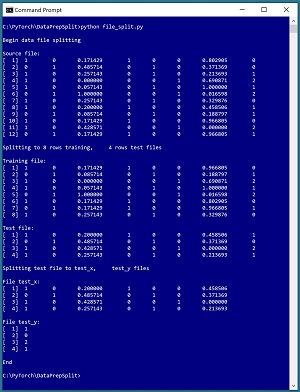
A good way to understand data file splitting and see where this article is headed is to take a look at the screenshot of a demo program in Figure 1. The demo uses a small 12-line text file named people_encoded.txt where each line represents one person. There are eight columns: two for encoded sex, one for normalized age, three for encoded region, one for normalized income, and one for encoded political leaning.
The data has been processed by removing missing values, editing bad data, normalizing the numeric age and income values, and encoding the sex and region predictor values using one-hot encoding, and encoding the political leaning values using ordinal encoding. (Note: some neural network libraries require one-hot encoding for multi-class dependent variables.)
 [Click on image for larger view.] Figure 1: Programmatically Splitting Data
The demo is a Python language program, but programmatically splitting data encoding can be implemented using any language. The first five lines of the demo source data are:
1   0    0.171429   1    0    0    0.802905   0
0   1    0.485714   0    1    0    0.371369   0
1   0    0.257143   0    1    0    0.213693   1
1   0    0.000000   0    0    1    0.690871   2
1   0    0.057143   0    1    0    1.000000   1
. . .
The demo begins by displaying the source data file. Next, the demo program loads the data into memory and shuffles the data into a random order. Then, the first 8 lines (75 percent of the 12-item source) of the shuffled data are written to a file named people_train.txt and the remaining 4 lines are written to a people_test.txt file.
In some scenarios, it's useful to split training and test files so that all the predictor values are in one file and all the dependent values-to-predict are in a second file. The demo program does this column-split for the people_test.txt file and displays the results.
This article assumes you have intermediate or better skill with a C-family programming language. The demo program is coded using Python but you shouldn't have too much trouble refactoring the demo code to another language if you wish. The complete source code for the demo program is presented in this article. The source code is also available in the accompanying file download.
The Data Preparation Pipeline
Although data preparation is different for every problem scenario, in general the data preparation pipeline for most ML systems usually follows something similar to the steps shown in Figure 2.
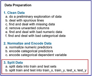 [Click on image for larger view.] Figure 2: Data Preparation Pipeline Typical Tasks
Data preparation for ML is deceptive because the process is conceptually easy. However, there are many steps, and each step is much more complicated than you might expect if you're new to ML. This article explains the tenth and eleventh steps in Figure 2. Other Data Science Lab articles explain the other seven steps. The data preparation series of articles can be found at https://visualstudiomagazine.com/Articles/List/Neural-Network-Lab.aspx.
The tasks in Figure 2 are usually not followed in a strictly sequential order. You often have to backtrack and jump around to different tasks. But it's a good idea to follow the steps shown in order as much as possible. For example, it's better to normalize and encode data before splitting the data into training and test files, because if you split first, then you have two files to normalize and encode instead of just one.
The Splitting Algorithm
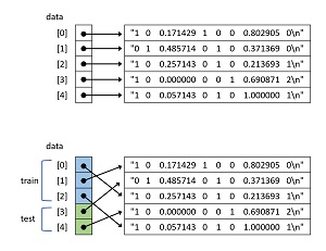
There are a surprising number of different ways to randomly split a file into two files. The technique used by the demo program is illustrated in Figure 3. The top images shows five lines of a source data file which have been read into memory as a NumPy array of string objects, including the newline terminator.
 [Click on image for larger view.] Figure 3: Splitting Algorithm Used by the Demo Program
The bottom image shows the data array after it has been shuffled. Notice that because references are being rearranged, the shuffle process is quick and efficient. After shuffling, the first 3 lines (60 percent) of data are designated as training items and can be written to one file, and the remaining 2 lines (40 percent) can be written to a file for test data.
A Python implementation of this technique is presented in Listing 1. Function file_split_rows() calls a program-defined helper function line_count() and uses a NumPy (aliased as np) array object. The function signature and first three statements are:
def file_split_rows(src, dest1, dest2, nrows1,
  rnd_order, seed=1):
  fin = open(src, "r")
  fout1 = open(dest1, "w")
  fout2 = open(dest2, "w")
. . .
The function has six parameters. The first three parameters (src, dest1, dest2) are string paths to the source file, the training file, and the test file.
The fourth parameter (nrows1) is the number of lines for the training file. An alternative design is to specify the percentage of lines to be used, such as 0.80 but I prefer to be explicit with regards to number of lines. The number of lines to be used for the test file is inferred. For example, if the source file has 1000 lines and parameter nrows1 is 800 then the number of lines for the test file must be 200. I usually use a parameter nrows2 and explicitly specify its value. I omit the nrows2 parameter in the demo program because the majority of external library implementations of file splitting functions I've seen use the implicit approach.
The fifth parameter (rnd_order) holds a Boolean value that controls whether to shuffle the source data or not. In most cases you'll set rnd_order=True to shuffle the data but you can set rnd_order=False if the source data has already been shuffled and you want to maintain the ordering. The sixth parameter (seed) is used to initialize a RandomState object which is local to the file_split_rows() function so that you can reproduce results.
Listing 1: Splitting by Rows
def file_split_rows(src, dest1, dest2, nrows1,
  rnd_order, seed=1):
  fin = open(src, "r")
  fout1 = open(dest1, "w")
  fout2 = open(dest2, "w")

  n = line_count(src)
  data = np.empty(n, dtype=np.object)
  i = 0
  for line in fin:
    data[i] = line
    i += 1
  fin.close()

  rnd = np.random.RandomState(seed)
  if rnd_order == True:
    rnd.shuffle(data)

  for i in range(0, nrows1):  # first nrows1 rows
    fout1.write(data[i])
  fout1.close()

  for i in range(nrows1, len(data)):  # remaining
    fout2.write(data[i])
  fout2.close()
Function file_split_rows() reads the source data into memory using these seven statements:
  n = line_count(src)
  data = np.empty(n, dtype=np.object)
  i = 0
  for line in fin:
    data[i] = line  # includes newline
    i += 1
  fin.close()
The total number of lines in the source data file is determined by a call to helper function line_count(). An alternative is to pass this value in as a parameter, the idea being that you should know the size of the source data. Another alternative is to omit the call to the line_count() function and compute the number of lines on-the-fly.
After the number of lines in the source file is known, that value is used to instantiate a NumPy array of type np.object. One of the quirks of NumPy is that if you want an array of strings you must use type np.object rather than type np.str as you might expect.
After the data is read into memory, the data is shuffled like so:
  rnd = np.random.RandomState(seed)
  if rnd_order == True:
    rnd.shuffle(data)
The built-in NumPy random.shuffle() function uses the Fisher-Yates algorithm to rearrange the references in its array argument. The function works by reference rather than by value so you don't need to write data = rnd.shuffle(data) although this statement would work too.
After the in-memory data has been shuffled, the first nrows1 of rows are written to the training file and the remaining (n - nrows1) rows are written to the test file:
  for i in range(0, nrows1):  # first nrows1 rows
    fout1.write(data[i])
  fout1.close()

  for i in range(nrows1, len(data)):  # remaining
    fout2.write(data[i])
  fout2.close()
As is often the case, you have to be careful for off-by-one errors because the Python range(start, end) function goes from start (inclusive) to end (exclusive).
Helper function line_count() is defined as:
def line_count(fn):
  ct = 0
  fin = open(fn, "r")
  for line in fin:
    ct += 1
  fin.close()
  return ct
The file is opened for reading and then traversed using a Python for-in idiom. Each line of the file, including the terminating newline character, is stored into variable named "line" but that variable isn't used. There are many alternative approaches.
The Demo Program
The structure of the demo program, with a few minor edits to save space, is shown in Listing 2. I indent my Python programs using two spaces, rather than the more common four spaces or a tab character, as a matter of personal preference. The program has four worker functions plus a main() function to control program flow. The purpose of worker functions show_file(), line_count(), file_split_rows(), and file_split_cols() should be clear from their names.
Listing 2: File Splitting Demo Program
# file_split.py
# Python 3.7.6

import numpy as np

def show_file(fn, start, end, indices=False,
 strip_nl=False): . . .

def line_count(fn): . . .

def file_split_rows(src, dest1, dest2, nrows1,
  rnd_order, seed=1): . . .

def file_split_cols(src, dest1, dest2,
  cols1, cols2, delim): . . .

def main():
  print("\nBegin data file splitting ")

  src = ".\\people_encoded.txt"
  dest1 = ".\\people_train.txt"
  dest2 = ".\\people_test.txt"

  print("\nSource file: ")
  show_file(src, start=1, end=-1,
    indices=True, strip_nl=True)

  print("\nSplitting to 8 rows training, \
    4 rows test files")
  file_split_rows(src, dest1, dest2, 8,
    rnd_order=True, seed=188)

  print("\nTraining file: ")
  show_file(dest1, 1, -1, indices=True,
    strip_nl=True)

  print("\nTest file: ")
  show_file(dest2, 1, -1, indices=True,
    strip_nl=True)

  print("\nSplitting test file to test_x, \
    test_y files ")
  src = ".\\people_test.txt"
  dest1 = ".\\people_test_x.txt"
  dest2 = ".\\people_test_y.txt"
  file_split_cols(src, dest1, dest2,
    [0,1,2,3,4,5,6], [7], "\t")

  print("\nFile test_x: ")
  show_file(dest1, 1, -1, indices=True,
    strip_nl=True)

  print("\nFile test_y: ")
  show_file(dest2, 1, -1, indices=True,
    strip_nl=True)

  print("\nEnd ")

if __name__ == "__main__":
  main()
The execution of the demo program begins with:
def main():
  print("\nBegin data file splitting ")
  src = ".\\people_encoded.txt"
  dest1 = ".\\people_train.txt"
  dest2 = ".\\people_test.txt"
  print("\nSource file: ")
  show_file(src, start=1, end=-1,
    indices=True, strip_nl=True)
  . . .
The entire source data file is displayed by a call to show_file() with arguments start=1 and end=-1. The -1 value is a special flag value that means "all lines". In most cases with large data files, you'll examine just a few lines of your data file rather than the entire file.
The indices=True argument instructs show_file() to display 1-based line numbers. With some data preparation tasks it's more natural to use 1-based indexing, but with other tasks it's more natural to use 0-based indexing. Either approach is OK but you've got to be careful of off-by-one errors. The strip_nl=True argument instructs function show_file() to remove trailing newlines from the data lines before printing them to the console shell so that there aren't blank lines between data lines in the display.
The demo continues with:
  print("\nSplitting to 8 rows training, \
    4 rows test files")
  file_split_rows(src, dest1, dest2, 8,
    rnd_order=True, seed=188)
  . . .