The Data Science Lab
Multi-Class Classification Using New PyTorch Best Practices, Part 2: Training, Accuracy, Predictions
Following new best practices, Dr. James McCaffrey of Microsoft Research revisits multi-class classification for when the variable to predict has three or more possible values.
This is the second of two articles that explain how to create and use a PyTorch multi-class classifier. A good way to see where this article is headed is to examine the screenshot of a demo program in Figure 1.
The demo program predicts the political leaning (conservative, moderate, liberal) of a person. The
first article
in the series explained how to prepare the training and test data, and how to define the neural network classifier. This article explains how to train the network, compute the accuracy of the trained network, use the network to make predictions, and save the network for use by other programs.
The demo begins by loading a 200-item file of training data and a 40-item set of test data. Each tab-delimited line represents a person. The fields are sex, age, state of residence (Michigan, Nebraska or Oklahoma), annual income and politics type (0 = conservative, 1 = moderate, 2 = liberal). The goal is to predict politics type from sex, age, state and income.
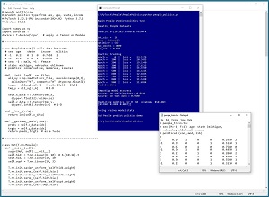 [Click on image for larger view.] Figure 1: Multi-Class Classification Using PyTorch Demo Run
After the training data is loaded into memory, the demo creates a 6-(10-10)-3 neural network. There are six input nodes, two hidden neural layers with 10 nodes each and three output nodes.
The demo prepares to train the network by setting a batch size of 10, stochastic gradient descent (SGD) optimization with a learning rate of 0.01, and maximum training epochs of 1,000 passes through the training data. The meaning of these values and how they are determined will be explained shortly.
The demo program monitors training by computing and displaying the loss value for one epoch. The loss value slowly decreases, which indicates that training is probably succeeding. The magnitude of the loss values isn't directly interpretable; the important thing is that the loss decreases.
After 1,000 training epochs, the demo program computes the accuracy of the trained model on the training data as 81.50 percent (163 out of 200 correct). The model accuracy on the test data is 75.00 percent (30 out of 40 correct).
After evaluating the trained network, the demo predicts the politics type for a person who is male, 30 years old, from Oklahoma and who makes $50,000 annually. The prediction is [0.6905, 0.3049, 0.0047]. These values are pseudo-probabilities. The largest value (0.6905) is at index [0] so the prediction is class 0 = conservative.
The demo concludes by saving the trained model to file so that it can be used without having to retrain the network from scratch. There are two different ways to save a PyTorch model. The demo uses the save-state approach.
This article assumes you have a basic familiarity with Python and intermediate or better experience with a C-family language but does not assume you know much about PyTorch or neural networks. The complete demo program source code and data can be found in my Sept. 1 post, "Multi-Class Classification Using PyTorch 1.12.1 on Windows 10/11."
As noted, the first article in this two-part series can be found in my Visual Studio Magazine Data Science Lab.
Overall Program Structure
The overall structure of the demo program is presented in Listing 1. The demo program is named people_politics.py. The program imports the NumPy (numerical Python) library and assigns it an alias of np. The program imports PyTorch and assigns it an alias of T. Most PyTorch programs do not use the T alias, but my work colleagues and I often do so to save space. The demo program indents using two spaces rather than the more common four spaces, again to save space.
Listing 1: Overall Program Structure
# people_politics.py
# predict politics type from sex, age, state, income
# PyTorch 1.12.1-CPU Anaconda3-2020.02  Python 3.7.6
# Windows 10/11

import numpy as np
import torch as T
device = T.device('cpu')

class PeopleDataset(T.utils.data.Dataset): . . .

class Net(T.nn.Module): . . .

def accuracy(model, ds): . . .

def main():
  # 0. get started
  print("Begin People predict politics type ")
  T.manual_seed(1)
  np.random.seed(1)

  # 1. create DataLoader objects
  # 2. create network
  # 3. train model
  # 4. evaluate model accuracy
  # 5. make a prediction
  # 6. save model (state_dict approach)

  print("End People predict politics demo")

if __name__ == "__main__":
  main()
The demo program places all the control logic in a main() function. Some of my colleagues prefer to implement a program-defined train() function to handle the code that performs the training.
Preparing to Train the Network
Training a neural network is the process of finding values for the weights and biases so that the network produces output that matches the training data. Most of the demo program code is associated with training the network. The terms network and model are often used interchangeably. In some development environments, network is used to refer to a neural network before it has been trained, and model is used to refer to a network after it has been trained.
In the main() function, the training and test data are loaded into memory as Dataset objects, and then the training Dataset is passed to a DataLoader object:
  # 1. create DataLoader objects
  print("Creating People Datasets ")

  train_file = ".\\Data\\people_train.txt"
  train_ds = PeopleDataset(train_file)  # 200 rows

  test_file = ".\\Data\\people_test.txt"
  test_ds = PeopleDataset(test_file)    # 40 rows

  bat_size = 10
  train_ldr = T.utils.data.DataLoader(train_ds,
    batch_size=bat_size, shuffle=True)
Unlike Dataset objects that must be defined for each specific multi-class problem, DataLoader objects are ready to use as-is. The batch size of 10 is a hyperparameter. The special case when batch size is set to 1 is sometimes called online training.
Although not necessary, it's generally a good idea to set a batch size that evenly divides the total number of training items so that all batches of training data have the same size. In the demo, with a batch size of 10 and 200 training items, each batch will have 20 items. When the batch size doesn't evenly divide the number of training items, the last batch will be smaller than all the others. The DataLoader class has an optional drop_last parameter with a default value of False. If set to True, the DataLoader will ignore last batches that are smaller.
It's very important to explicitly set the shuffle parameter to True. The default value is False. When shuffle is set to True, the training data will be served up in a random order which is what you want during training. If shuffle is set to False, the training data is served up sequentially. This almost always results in failed training because the updates to the network weights and biases oscillate, and no progress is made.
Creating the Network
The demo program creates the neural network like so:
  # 2. create network
  print("Creating 6-(10-10)-3 neural network ")
  net = Net().to(device)
  net.train()
The neural network is instantiated using normal Python syntax but with .to(device) appended to explicitly place storage in either "cpu" or "cuda" memory. Recall that device is a global-scope value set to "cpu" in the demo.
The network is set into training mode with the somewhat misleading statement net.train(). PyTorch neural networks can be in one of two modes, train() or eval(). The network should be in train() mode during training and eval() mode at all other times.
The train() vs. eval() mode is often confusing for people who are new to PyTorch in part because in many situations it doesn't matter what mode the network is in. Briefly, if a neural network uses dropout or batch normalization, then you get different results when computing output values depending on whether the network is in train() or eval() mode. But if a network doesn't use dropout or batch normalization, you get the same results for train() and eval() mode.
Because the demo network doesn't use dropout or batch normalization, it's not necessary to switch between train() and eval() modes. However, in my opinion it's good practice to always explicitly set a network to train() mode during training and eval() mode at all other times. By default, a network is in train() mode.
The statement net.train() is rather misleading because it suggests that some sort of training is going on. If I had been the person who implemented the train() method, I would have named it set_train_mode() instead. Also, the train() method operates by reference and so the statement net.train() modifies the net object. If you are a fan of functional programming, this will probably make you want to tear your hair out, and you can write net = net.train() instead.
Training the Network
The code that trains the network is presented in Listing 2. Training a neural network involves two nested loops. The outer loop iterates a fixed number of epochs (with a possible short-circuit exit). An epoch is one complete pass through the training data. The inner loop iterates through all training data items.
Listing 2: Training the Network
  # 3. train model
  max_epochs = 1000
  ep_log_interval = 100
  lrn_rate = 0.01

  loss_func = T.nn.NLLLoss()  # assumes log_softmax()
  optimizer = T.optim.SGD(net.parameters(),
    lr=lrn_rate)

  print("bat_size = %3d " % bat_size)
  print("loss = " + str(loss_func))
  print("optimizer = SGD")
  print("max_epochs = %3d " % max_epochs)
  print("lrn_rate = %0.3f " % lrn_rate)

  print("Starting training ")
  for epoch in range(0, max_epochs):
    # T.manual_seed(epoch+1)  # reproducibility
    epoch_loss = 0  # for one full epoch

    for (batch_idx, batch) in enumerate(train_ldr):
      X = batch[0]  # inputs
      Y = batch[1]  # correct class/label/politics

      optimizer.zero_grad()
      oupt = net(X)
      loss_val = loss_func(oupt, Y)  # a tensor
      epoch_loss += loss_val.item()  # accumulate
      loss_val.backward()
      optimizer.step()

    if epoch % ep_log_interval == 0:
      print("epoch = %5d  |  loss = %10.4f" % \
        (epoch, epoch_loss))
  print("Training done ")
The five statements that prepare training are:
  max_epochs = 1000
  ep_log_interval = 100
  lrn_rate = 0.01
  loss_func = T.nn.NLLLoss()
  optimizer = T.optim.SGD(net.parameters(),
    lr=lrn_rate)
The number of epochs to train is a hyperparameter that must be determined by trial and error. The ep_log_interval specifies how often to display progress messages.
The loss function is set to NLLLoss(), which assumes that the output nodes have log_softmax() activation applied. There is a strong coupling between loss function and output node activation.
The demo uses stochastic gradient descent optimization (SGD) with a learning rate of 0.01, which controls how much weights and biases change on each update. PyTorch supports 13 different optimization algorithms. The two most common are SGD and Adam (adaptive moment estimation). SGD often works reasonably well for simple networks, including multi-class classifiers. Adam often works better than SGD for deep neural networks.
PyTorch beginners often fall down a technical rabbit hole trying to learn everything about every optimization algorithm. Most of my experienced colleagues use just two or three algorithms and adjust the learning rate. My recommendation is to use SGD and Adam and try other algorithms only when those two fail.
It's important to monitor training progress because training failure is the norm rather than the exception. There are several ways to monitor training progress. The demo program uses the simplest approach which is to accumulate the total loss for one epoch, and then display that accumulated loss value every so often (ep_log_interval = 100 in the demo).
The inner training loop is where all the work is done:
  for (batch_idx, batch) in enumerate(train_ldr):
    X = batch[0]  # inputs
    Y = batch[1]  # correct class/label/politics
    optimizer.zero_grad()
    oupt = net(X)
    loss_val = loss_func(oupt, Y)  # a tensor
    epoch_loss += loss_val.item()  # accumulate
    loss_val.backward()
    optimizer.step()
The enumerate() function returns the current batch index (0 through 19) and a batch of input values (sex, age, state, income) with associated correct target values (0, 1 or 2). Using enumerate() is optional and you can skip getting the batch index by writing "for batch in train_ldr" instead.
The NLLLoss() loss function returns a PyTorch tensor that holds a single numeric value. That value is extracted using the item() method so it can be accumulated as an ordinary non-tensor numeric value. In early versions of PyTorch, using the item() method was required, but newer versions of PyTorch perform an implicit type-cast so the call to item() is not necessary. In my opinion, explicitly using the item() method is better coding style.
The backward() method computes gradients. Each weight and bias has an associated gradient. Gradients are numeric values that indicate how an associated weight or bias should be adjusted so that the error/loss between computed outputs and target outputs is reduced. It's important to remember to call the zero_grad() method before calling the backward() method. The step() method uses the newly computed gradients to update the network weights and biases.