The Data Science Lab
Positive and Unlabeled Learning (PUL) Using PyTorch
Dr. James McCaffrey of Microsoft Research provides a code-driven tutorial on PUL problems, which often occur with security or medical data in cases like training a machine learning model to predict if a hospital patient has a disease or not.
A positive and unlabeled learning (PUL) problem occurs when a machine learning set of training data has only a few positive labeled items and many unlabeled items. PUL problems often occur with security or medical data. For example, suppose you want to train a machine learning model to predict if a hospital patient has a disease or not, based on predictor variables such as age, blood pressure, and so on. The training data might have a few dozen instances of items that are positive (class 1 = patient has disease) and many hundreds or thousands of instances of data items that are unlabeled and so could be either class 1 = patient has disease, or class 0 = patient does not have disease.
The goal of PUL is to use the information contained in the dataset to guess the true labels of the unlabeled data items. After the class labels of some of the unlabeled items have been guessed, the resulting labeled dataset can be used to train a binary classification model using any standard machine learning technique, such as k-nearest neighbors classification, neural binary classification, logistic regression classification, naive Bayes classification, and so on.
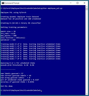
A good way to see where this article is headed is to take a look at the screenshot of a demo program in Figure 1. The demo uses a 200-item dataset of employee information where the ultimate goal is to classify an employee as an introvert (class 0) or an extrovert (class 1). The dataset is positive and unlabeled: there are just 20 positive (extrovert) employees but the remaining 180 employees are unlabeled and could be either introvert or extrovert.
PUL is challenging and there are several techniques to tackle such problems. The demo program repeatedly (eight times) trains a helper binary classifier using the 20 positive employee data items and 20 randomly selected unlabeled items which are temporarily treated as negative. During the eight model training sessions, information about the unused, unlabeled employee data items is accumulated, in a way that will be explained shortly.
After the eight models have been trained and analyzed, the accumulated information is used to guess the true labels of some of the 180 unlabeled employees. Based on two user-supplied threshold values of 0.30 and 0.90, the PUL system believes it has enough evidence to make intelligent guesses for 57 of the 180 unlabeled employees (32 percent of them).
The true class labels for all 200 employees is known by the demo system. Of the 57 class label guesses, 49 were correct and 8 were incorrect (86 percent accuracy). The demo does not continue by using the now-labeled 97 employee data items (the original 20 positive labeled plus the 57 newly labeled) to create a binary classifier, but that would be the next step in a non-demo scenario.
 [Click on image for larger view.] Figure 1: Positive and Unlabeled Learning (PUL) in Action
This article assumes you have an intermediate or better familiarity with a C-family programming language, preferably Python, and a basic familiarity with the PyTorch code library. The source code for the demo program is a bit too long to present in its entirety in this article, but the complete code and training data are available in the accompanying file download. (The PUL data is embedded in commented-form into the source code).
This article focuses on explaining the key ideas you need to understand in order to analyze and process PUL data to suit your problem scenarios. All normal error checking code has been omitted to keep the main ideas as clear as possible.
To run the demo program, you must have Python and PyTorch installed on your machine. The demo programs were developed on Windows 10 using the Anaconda 2020.02 64-bit distribution (which contains Python 3.7.6) and PyTorch version 1.8.0 for CPU installed via pip. Installation is not trivial. You can find detailed step-by-step installation instructions for this configuration in my blog post.
The PUL Employee Data
The data file of employee information has 200 tab-delimited items. The data looks like:
-2   0.39   0   0   1   0.5120   0   1   0
 1   0.24   1   0   0   0.2950   0   0   1
-2   0.36   1   0   0   0.4450   0   1   0
-2   0.50   0   1   0   0.5650   0   1   0
-2   0.19   0   0   1   0.3270   1   0   0
. . .
The first column is introvert or extrovert, encoded as 1 = positive = extrovert (20 items), and -2 = unlabeled (180 items). The goal of PUL is to intelligently guess 0 = negative, or 1 = positive, for as many of the unlabeled data items as possible.
The other columns in the dataset are employee age (normalized by dividing by 100), city (one of three, one-hot encoded), annual income (normalized by dividing by $100,000), and job-type (one of three, one-hot encoded).
The dataset was artificially constructed so that even numbered items [0], [2], [4], etc. are actually class 0 = negative, and odd numbered items [1], [3], [5], etc. are actually class 1. This allows the PUL system to measure its accuracy. In a non-demo PUL scenario, you usually won't know the true class labels.
The PUL Algorithm
The technique presented in this article is based on a 2013 research paper by F. Mordelet and J.P. Vert, titled "A Bagging SVM to Learn from Positive and Unlabeled Examples". That paper uses a SVM (support vector machine) binary classifier to analyze unlabeled data. This article uses a neural binary classifier instead.
In pseudo-code:
create a 40-item train dataset with all 20 positive
  and 20 randomly selected unlabeled items that
  are temporarily treated as negative

loop several times
  train a binary classifier using the 40-item train data
  use trained model to score the 160 unused unlabeled
    data items
  accumulate the p-score for each unused unlabeled item

  generate a new train dataset with the 20 positive
    and 20 different unlabeled items treated as negative
end-loop


for-each of the 180 unlabeled items
  compute the average p-value

  if avg p-value < lo threshold
    guess its label as negative
  else-if avg p-value > hi threshold
    guess its label as positive
  else
    insufficient evidence to make a guess
  end-if
end-for
Each time through the training loop, the binary classifier will make fairly poor predictions but the average prediction for all iterations will likely be good. Recall that a neural binary classifier will predict by generating a p-value (pseudo-probability) between 0.0 and 1.0 where a p-value less than 0.5 indicates class 0 = negative, and a p-value greater than 0.5 indicates class 1 = positive. Suppose that an unlabeled data item is not used as part of the training data, three times. And suppose that the trained model scores that unlabeled data item as 0.65, 0.22, 0.58 which mean that the unlabeled item was predicted to be class 1 = positive twice, and class 0 = negative once. The average p-value for the item is (0.65 + 0.32 + 0.78) / 3 = 0.58. Because the average p-value of the unlabeled item is greater than 0.5, it is most likely class 1 = positive.
If you use a decision threshold of 0.5, every unlabeled data item will be guessed as positive or negative. However, many of the guesses where the average p-value is close to 0.5 will likely be incorrect. An alternative approach taken by the demo is to only guess labels where the average p-value is below a low threshold (0.3) or above a high threshold (0.90). Items with average p-values between 0.30 and 0.90 are judged to be ambiguous so no label is guessed.
The low and high threshold values are system hyperparameters that must be determined by the nature of your problem scenario. Adjusting the threshold values towards 0.5 will increase the number of guesses for the unlabeled data items, but probably decrease the accuracy of those guesses.
Generating a Dynamic Dataset
Somewhat unexpectedly, the most difficult part of a PUL system is wrangling the data to generate dynamic (changing) training datasets. The challenge is to be able to create an initial training dataset with the 20 positive items and 20 randomly selected unlabeled items like so:
train_file = ".\\Data\\employee_pul_200.txt"
train_ds = EmployeeDataset(train_file, 20, 180)
And then inside a loop, be able to reinitialize the training dataset with the same 20 positive items but 20 different unlabeled items:
train_ds.reinit()
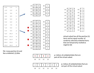
The dynamic dataset architecture used by the demo program is illustrated in Figure 2. The diagram shows a 14-item dummy PUL dataset with four positive items and ten unlabeled items rather than the 200-item demo dataset. The source PUL data is read into memory as four Python lists of arrays. The first two lists hold the predictors and labels for the four positive items. Note that the positive labels don't need to be explicitly stored because they're all 1, but explicit storage make the code easier to work with. The second two lists hold the predictors and labels for the more numerous unlabeled items, where the unlabeled classes are temporarily all marked as class 0 = negative.
 [Click on image for larger view.] Figure 2: A Dynamic Virtual Dataset for PUL
Each dynamic dataset needs all four of the positive items and four randomly selected unlabeled-marked-as-negative items. It would be inefficient to duplicate data, so all that's needed is information about which rows of the data in memory belong to the positive items and which rows belong to the unlabeled-negative items. And because all positive items are always used in each dynamic dataset, the only information needed is the four rows of unlabeled-negative that are in the dynamic dataset ([6], [3], [8], [2]), and which six rows are not part of the dynamic dataset ([0], [1], [4], [5], [7], [9]).
The virtual dynamic dataset has size 8. To fetch a specified item from it, if the requested index is between [0] and [3] the item can be accessed directly because it must be a positive item. For example, to get the predictor values for virtual item [2], [2] is fetched from memory giving (7.0, 8.0) from Figure 2.
If the requested index is greater than [3] then the requested index must be mapped to its location in memory. For example, to get virtual item [6], the 6 is mapped by subtracting 4 (number of unlabeled-negative items), giving [2]. That value is used to look into the p array that stores memory locations, giving [8] from Figure 2. Item [8] is looked up in memory giving predictor values (11.0, 12.0).
The key takeaway is that PUL systems are not trivial. You must spend a significant amount of engineering time and effort to deal with data wrangling.
The demo code that implements a dynamic virtual dataset for the employee PUL data is presented in Listing 1. As is often the case, data wrangling code is tedious and tricky.
Listing 1: Defining a Dynamic Dataset for PUL Data
class EmployeeDataset(T.utils.data.Dataset):
  # label  age   city   income   job-type
  #   1    0.39  1 0 0  0.5432   1 0 0
  #  -2    0.29  0 0 1  0.4985   0 1 0  (unlabeled)
  # . . .
  #  [0]   [1]  [2 3 4]   [5]   [6 7 8]

  def __init__(self, fn, tot_num_pos, tot_num_unl):
    self.rnd = np.random.RandomState(1)

    self.tot_num_pos = tot_num_pos  # number positives
    self.tot_num_unl = tot_num_unl  # num unlabeleds

    pos_x_lst = []; pos_y_lst = []  # lists of vectors
    unl_x_lst = []; unl_y_lst = []

    ln = 0  # line number (not including comments)
    j = 0  # counter for unlabeleds

    self.unl_idx_to_line_num = dict()
    # key = idx of an unlabeled item in memory,
    # val = corresponding line number in src data file

    fin = open(fn, "r")  # four lists of arrays
    for line in fin:
      line = line.strip()
      if line.startswith("#"): continue

      arr = np.fromstring(line, sep="\t", \
        dtype=np.float32)
      if arr[0] == 1:
        pos_x = arr[[1,2,3,4,5,6,7,8]]
        pos_y = 1  # always 1
        pos_x_lst.append(pos_x)
        pos_y_lst.append(pos_y)
      elif arr[0] == -2:  # unlabeled
        unl_x = arr[[1,2,3,4,5,6,7,8]]
        unl_y = 0  # treat unlabeleds as negative
        unl_x_lst.append(unl_x)
        unl_y_lst.append(unl_y)
        self.unl_idx_to_line_num[j] = ln
        j +=1
      else:
        print("Fatal: unknown label in file")

      ln += 1  # only data lines

    fin.close()

    # data actual storage in 4 tensor-arrays
    self.train_x_pos = T.tensor(pos_x_lst, \
      dtype=T.float32) # predictors for positives
    self.train_y_pos = T.tensor(pos_y_lst, \
      dtype=T.float32).reshape(-1,1) # positives (1s)
    self.train_x_unl = T.tensor(unl_x_lst, \
      dtype=T.float32) # predictors for unlabels
    self.train_y_unl = T.tensor(unl_y_lst, \
      dtype=T.float32).reshape(-1,1)

    self.num_pos_unl = 2 * tot_num_pos

    # indices of active and inactive unlabeled items
    all_unl_indices = np.arange(tot_num_unl)  # 180
    self.rnd.shuffle(all_unl_indices)
    self.p = all_unl_indices[0 : tot_num_pos]  # 20
    self.q = all_unl_indices[tot_num_pos : tot_num_unl]

  def __len__(self):
    return self.num_pos_unl  # virtual ds size

  def __getitem__(self, idx):
    if idx < self.tot_num_pos:  # small: fetch directly
      return (self.train_x_pos[idx], self.train_y_pos[idx])
    else:   # large index = an unlabeled = map index
      ofset = idx - self.tot_num_pos
      ii = self.p[ofset]  # index of active unlabeled item
      return (self.train_x_unl[ii], self.train_y_unl[ii])

  def reinit(self):  # get (20) different unlabeled items
    all_unl_indices = np.arange(self.tot_num_unl)
    self.rnd.shuffle(all_unl_indices)
    self.p = all_unl_indices[0 : self.tot_num_pos]
    self.q = all_unl_indices[self.tot_num_pos : \
      self.tot_num_unl]