The Data Science Lab
CIFAR-10 Image Classification Using PyTorch
CIFAR-10 problems analyze crude 32 x 32 color images to predict which of 10 classes the image is. Here, Dr. James McCaffrey of Microsoft Research shows how to create a PyTorch image classification system for the CIFAR-10 dataset.
This article explains how to create a PyTorch image classification system for the CIFAR-10 dataset. CIFAR-10 images are crude 32 x 32 color images of 10 classes such as "frog" and "car." A good way to see where this article is headed is to take a look at the screenshot of a demo program in Figure 1. The demo begins by loading a 5,000-item subset of the 50,000-item CIFAR-10 training data, and a 1,000-item subset of the test data.
The demo program creates a convolutional neural network (CNN) that has two convolutional layers and three linear layers. The demo program trains the network for 100 epochs. An epoch is one pass through all training items. The loss/error values slowly decrease and the classification accuracy slowly increases, which indicates that training is probably working.
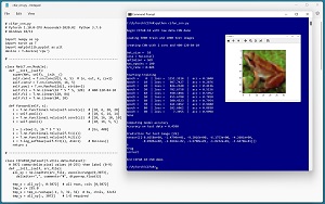 [Click on image for larger view.]Figure 1: CIFAR-10 Image Classification Using PyTorch Demo Run
After training, the demo program computes the classification accuracy of the model on the test data as 45.90 percent = 459 out of 1,000 correct. The classification accuracy is better than random guessing (which would give about 10 percent accuracy) but isn't very good mostly because only 5,000 of the 50,000 training images were used. A model using all training data can get about 90 percent accuracy on the test data.
Next, the trained model is used to predict the class label for a specific test item. The demo displays the image, then feeds the image to the trained model and displays the 10 output logit values. The largest of these values is -0.016942 which is at index location [6], which corresponds to class "frog." This is a correct prediction.
This article assumes you have a basic familiarity with Python and the PyTorch neural network library. If you're new to PyTorch, you can get up to speed by reviewing the article "Multi-Class Classification Using PyTorch: Defining a Network."
To run the demo program, you must have Python and PyTorch installed on your machine. The demo programs were developed on Windows 10/11 using the Anaconda 2020.02 64-bit distribution (which contains Python 3.7.6) and PyTorch version 1.10.0 for CPU installed via pip. You can find detailed step-by-step installation instructions for this configuration in my blog post.
The complete demo program source code is presented in this article. The source code is also available in the accompanying file download. Getting the CIFAR-10 data is not trivial because it's stored in compressed binary form rather than text. See "Preparing CIFAR Image Data for PyTorch."
The CIFAR-10 Data
The full CIFAR-10 (Canadian Institute for Advanced Research, 10 classes) dataset has 50,000 training images and 10,000 test images. Each image is 32 x 32 pixels. Because the images are color, each image has three channels (red, green, blue). Each pixel-channel value is an integer between 0 and 255. Figure 2 shows four of the CIFAR-10 training images.
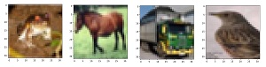 [Click on image for larger view.]Figure 2: Example CIFAR-10 Images
Each image is one of 10 classes: plane (class 0), car, bird, cat, deer, dog, frog, horse, ship, truck (class 9). Most neural network libraries, including PyTorch, scikit, and Keras, have built-in CIFAR-10 datasets. However, working with pre-built CIFAR-10 datasets has two big problems. First, a pre-built dataset is a black box that hides many details that are important if you ever want to work with real image data. Second, the pre-built datasets consist of all 50,000 training and 10,000 test images and those datasets are very difficult to work with because they're so large.
The demo program assumes the existence of a comma-delimited text file of 5,000 training images. Each image is stored on one line with the 32 * 32 * 3 = 3,072 pixel-channel values first, and the class "0" to "9" label last.
The Demo Program
The complete CIFAR-10 classification program, with a few minor edits to save space, is presented in Listing 1. I prefer to indent my Python programs with two spaces rather than the more common four spaces. The backslash character is used for line continuation in Python. Notepad is my text editor of choice but you can use any editor.
Listing 1: CIFAR-10 Demo Program
# cifar_cnn.py
# PyTorch 1.10.0-CPU Anaconda3-2020.02  Python 3.7.6
# Windows 10/11

import numpy as np
import torch as T
import matplotlib.pyplot as plt
device = T.device('cpu')

# -----------------------------------------------------------

class Net(T.nn.Module):
  def __init__(self):
    super(Net, self).__init__()
    self.conv1 = T.nn.Conv2d(3, 6, 5)  # in, out, k, (s=1)
    self.conv2 = T.nn.Conv2d(6, 16, 5)
    self.pool = T.nn.MaxPool2d(2, stride=2)
    self.fc1 = T.nn.Linear(16 * 5 * 5, 120)  # 400-120-84-10
    self.fc2 = T.nn.Linear(120, 84)
    self.fc3 = T.nn.Linear(84, 10)

  def forward(self, x):
    z = T.nn.functional.relu(self.conv1(x))  # [10, 6, 28, 28]
    z = self.pool(z)                         # [10, 6, 14, 14]
    z = T.nn.functional.relu(self.conv2(z))  # [10, 16, 10, 10]
    z = self.pool(z)                         # [10, 16, 5, 5]

    z = z.reshape(-1, 16 * 5 * 5)            # [bs, 400]
    z = T.nn.functional.relu(self.fc1(z))
    z = T.nn.functional.relu(self.fc2(z))
    z = T.log_softmax(self.fc3(z), dim=1)    # NLLLoss()
    return z

# -----------------------------------------------------------

class CIFAR10_Dataset(T.utils.data.Dataset):
  # 3072 comma-delim pixel values (0-255) then label (0-9)
  def __init__(self, src_file):
    all_xy = np.loadtxt(src_file, usecols=range(0,3073),
      delimiter=",", comments="#", dtype=np.float32)

    tmp_x = all_xy[:, 0:3072]  # all rows, cols [0,3072]
    tmp_x /= 255.0
    tmp_x = tmp_x.reshape(-1, 3, 32, 32)  # bs, chnls, 32x32
    tmp_y = all_xy[:, 3072]    # 1-D required

    self.x_data = \
      T.tensor(tmp_x, dtype=T.float32).to(device)
    self.y_data = \
      T.tensor(tmp_y, dtype=T.int64).to(device)

  def __len__(self):
    return len(self.x_data)

  def __getitem__(self, idx):
    lbl = self.y_data[idx]
    pixels = self.x_data[idx]
    return (pixels, lbl)

# -----------------------------------------------------------

def accuracy(model, ds):
  X = ds[0:len(ds)][0]  # all images
  Y = ds[0:len(ds)][1]  # all targets
  with T.no_grad():
    logits = model(X)
  predicteds = T.argmax(logits, dim=1)
  num_correct = T.sum(Y == predicteds)
  acc = (num_correct * 1.0) / len(ds)
  return acc.item()

# -----------------------------------------------------------

def main():
  # 0. setup
  print("\nBegin CIFAR-10 with raw data CNN demo ")
  np.random.seed(1)
  T.manual_seed(1)

  # 1. create Dataset
  print("\nLoading 5000 train and 1000 test images ")
  train_file = ".\\Data\\cifar10_train_5000.txt"
  train_ds = CIFAR10_Dataset(train_file)
  test_file = ".\\Data\\cifar10_test_1000.txt"
  test_ds = CIFAR10_Dataset(test_file)

  bat_size = 10
  train_ldr = T.utils.data.DataLoader(train_ds,
    batch_size=bat_size, shuffle=True)

  # 2. create network
  print("\nCreating CNN with 2 conv and 400-120-84-10 ")
  net = Net().to(device)

# -----------------------------------------------------------

  # 3. train model
  max_epochs = 100
  ep_log_interval = 10
  lrn_rate = 0.005

  loss_func = T.nn.NLLLoss()  # log-softmax() activation
  optimizer = T.optim.SGD(net.parameters(), lr=lrn_rate)

  print("\nbat_size = %3d " % bat_size)
  print("loss = " + str(loss_func))
  print("optimizer = SGD")
  print("max_epochs = %3d " % max_epochs)
  print("lrn_rate = %0.3f " % lrn_rate)

  print("\nStarting training")
  net.train()
  for epoch in range(0, max_epochs):
    epoch_loss = 0  # for one full epoch
    for (batch_idx, batch) in enumerate(train_ldr):
      (X, Y) = batch  # X = pixels, Y = target labels
      optimizer.zero_grad()
      oupt = net(X)  # X is Size([bat_size, 3, 32, 32])
      loss_val = loss_func(oupt, Y)  # a tensor
      epoch_loss += loss_val.item()  # accumulate
      loss_val.backward()
      optimizer.step()
    if epoch % ep_log_interval == 0:
      print("epoch = %4d  | loss = %10.4f  | " % \
        (epoch, epoch_loss), end="")
      net.eval()
      acc = accuracy(net, train_ds)
      net.train()
      print(" acc = %6.4f " % acc)
  print("Done ")

# -----------------------------------------------------------

  # 4. evaluate model accuracy
  print("\nComputing model accuracy")
  net.eval()
  acc_test = accuracy(net, test_ds)  # all at once
  print("Accuracy on test data = %0.4f" % acc_test)

  # 5. TODO: save trained model

# -----------------------------------------------------------

  # 6. use model to make a prediction
  print("\nPrediction for test image [29] ")
  img = test_ds[29][0]
  label = test_ds[29][1]

  img_np = img.numpy()  # 3,32,32
  img_np = np.transpose(img_np, (1, 2, 0))
  plt.imshow(img_np)
  plt.show()

  labels = ['plane', 'car', 'bird', 'cat', 'deer', 'dog',
    'frog', 'horse', 'ship', 'truck']
  img = img.reshape(1, 3, 32, 32)  # make it a batch
  with T.no_grad():
    logits = net(img)
  y = T.argmax(logits)  # 0 to 9 as a tensor
  print(logits)         # 10 values
  print(y.item())
  print(labels[y.item()])  # like "frog"

  if y.item() == label.item():
    print("correct")
  else:
    print("wrong")

  print("\nEnd CIFAR-10 CNN demo ")

if __name__ == "__main__":
  main()
All the control logic is in a program-defined main() function. The class that defines a convolutional neural network uses two convolution layers with max-pooling followed by three linear layers. The neural network definition begins by defining six layers in the __init__() method:
import torch as T
class Net(T.nn.Module):
  def __init__(self):
    super(Net, self).__init__()
    self.conv1 = T.nn.Conv2d(3, 6, 5)  # in, out, k, (s=1)
    self.conv2 = T.nn.Conv2d(6, 16, 5)
    self.pool = T.nn.MaxPool2d(2, stride=2)
    self.fc1 = T.nn.Linear(16 * 5 * 5, 120)  # 400-120-84-10
    self.fc2 = T.nn.Linear(120, 84)
    self.fc3 = T.nn.Linear(84, 10)
. . .
Dealing with the geometries of the data objects is tricky. The first convolution layer accepts a batch of images with three physical channels (RGB) and outputs data with six virtual channels, The layer uses a kernel map of size 5 x 5, with a default stride of 1. This means each block of 5 x 5 values is combined to produce a new value. Convolution helps by taking into account the two-dimensional geometry of an image and gives some flexibility to deal with image translations such as a shift of all pixel values to the right. A stride of 1 shifts the kernel map one pixel to the right after each calculation, or one pixel down at the end of a row. The kernel map size and its stride are hyperparameters (values that must be determined by trial and error).
The second convolution layer accepts data with six channels (from the first convolution layer) and outputs data with 16 channels. The second convolution also uses a 5 x 5 kernel map with stride of 1. The output data has a total of 16 * 5 * 5 = 400 values. These 400 values are fed to the first linear layer fc1 ("fully connected 1"), which outputs 120 values. The 120 is a hyperparameter.
The second linear layer accepts the 120 values from the first linear layer and outputs 84 values. The third linear layer accepts those 84 values and outputs 10 values, where each value represents the likelihood of the 10 image classes. To summarize, an input image has 32 * 32 * 3 = 3,072 values. The image is fed to the convolutional network which produces 10 values where the index of the largest value represents the predicted class.
The network uses a max-pooling layer with kernel shape 2 x 2 and a stride of 2. This means each 2 x 2 block of values is replaced by the largest of the four values. Like convolution, max-pooling gives some ability to deal with image position shifts. Additionally, max-pooling gives some defense to model over-fitting.
The forward() method of the neural network definition uses the layers defined in the __init__() method:
  def forward(self, x):
    z = T.nn.functional.relu(self.conv1(x))  # [10, 6, 28, 28]
    z = self.pool(z)                         # [10, 6, 14, 14]
    z = T.nn.functional.relu(self.conv2(z))  # [10, 16, 10, 10]
    z = self.pool(z)                         # [10, 16, 5, 5]

    z = z.reshape(-1, 16 * 5 * 5)            # [bs, 400]
    z = T.nn.functional.relu(self.fc1(z))
    z = T.nn.functional.relu(self.fc2(z))
    z = T.log_softmax(self.fc3(z), dim=1)    # NLLLoss()
    return z
Using a batch size of 10, the data object holding the input images has shape [10, 3, 32, 32]. After applying the first convolution layer, the internal representation is reduced to shape [10, 6, 28, 28]. The max pool layer reduces the size of the batch to [10, 6, 14, 14]. The second convolution layer yields a representation with shape [10, 6, 10, 10]. The second application of max-pooling results in data with shape [10, 16, 5, 5].
This data is reshaped to [10, 400]. The code uses the special reshape -1 syntax which means, "all that's left." This is slightly preferable to using a hard-coded 10 because the last batch in an epoch might be smaller than all the others if the batch size does not evenly divide the size of the dataset.
In theory, all the shapes of the intermediate data representations can be computed by hand, but in practice it's faster to place print(z.shape) statements in the forward() method during development.