The Data Science Lab
Multi-Class Classification Using PyTorch: Defining a Network
Dr. James McCaffrey of Microsoft Research explains how to define a network in installment No. 2 of his four-part series that will present a complete end-to-end production-quality example of multi-class classification using a PyTorch neural network.
The goal of a multi-class classification problem is to predict a value that can be one of three or more possible discrete values, such as "red," "yellow" or "green" for a traffic signal. This article is the second in a series of four articles that present a complete end-to-end production-quality example of multi-class classification using a PyTorch neural network. The example problem is to predict a college student's major ("finance," "geology" or "history") from their sex, number of units completed, home state and score on an admission test.
The process of creating a PyTorch neural network multi-class classifier consists of six steps:
- Prepare the training and test data
- Implement a Dataset object to serve up the data
- Design and implement a neural network
- Write code to train the network
- Write code to evaluate the model (the trained network)
- Write code to save and use the model to make predictions for new, previously unseen data
A good way to see where this series of articles is headed is to take a look at the screenshot of the demo program in Figure 1. The demo begins by creating Dataset and DataLoader objects which have been designed to work with the student data. Next, the demo creates a 6-(10-10)-3 deep neural network. The demo prepares training by setting up a loss function (cross entropy), a training optimizer function (stochastic gradient descent) and parameters for training (learning rate and max epochs).
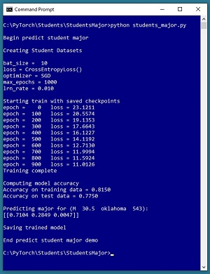 [Click on image for larger view.] Figure 1: Predicting Student Major Multi-Class Classification in Action
The demo trains the neural network for 1,000 epochs in batches of 10 items. An epoch is one complete pass through the training data. The training data has 200 items, therefore, one training epoch consists of processing 20 batches of 10 training items.
During training, the demo computes and displays a measure of the current error (also called loss) every 100 epochs. Because error slowly decreases, it appears that training is succeeding. This is good because training failure is usually the norm rather than the exception. Behind the scenes, the demo program saves checkpoint information after every 100 epochs so that if the training machine crashes, training can be resumed without having to start from the beginning.
After training the network, the demo program computes the classification accuracy of the model on the training data (163 out of 200 correct = 81.50 percent) and on the test data (31 out of 40 correct = 77.50 percent). Because the two accuracy values are similar, it's likely that model overfitting has not occurred. After evaluating the trained model, the demo program saves the model using the state dictionary approach, which is the most common of three standard techniques.
The demo concludes by using the trained model to make a prediction. The raw input is (sex = "M", units = 30.5, state = "oklahoma", score = 543). The raw input is normalized and encoded as (sex = -1, units = 0.305, state = 0, 0, 1, score = 0.5430). The computed output vector is [0.7104, 0.2849, 0.0047]. These values represent the pseudo-probabilities of student majors "finance", "geology" and "history" respectively. Because the probability associated with "finance" is the largest, the predicted major is "finance."
This article assumes you have an intermediate or better familiarity with a C-family programming language, preferably Python, but doesn't assume you know very much about PyTorch. The complete source code for the demo program, and the two data files used, are available in the download that accompanies this article. All normal error checking code has been omitted to keep the main ideas as clear as possible.
To run the demo program, you must have Python and PyTorch installed on your machine. The demo programs were developed on Windows 10 using the Anaconda 2020.02 64-bit distribution (which contains Python 3.7.6) and PyTorch version 1.7.0 for CPU installed via pip. Installation is not trivial. You can find detailed step-by-step installation instructions for this configuration at my blog.
The Student Data
The raw Student data is synthetic and was generated programmatically. There are a total of 240 data items, divided into a 200-item training dataset and a 40-item test dataset. The raw data looks like:
M  39.5  oklahoma  512  geology
F  27.5  nebraska  286  history
M  22.0  maryland  335  finance
. . .
M  59.5  oklahoma  694  history
Each line of tab-delimited data represents a hypothetical student at a hypothetical college. The fields are sex, units-completed, home state, admission test score and major. The first four values on each line are the predictors (often called features in machine learning terminology) and the fifth value is the dependent value to predict (often called the class or the label). For simplicity, there are just three different home states, and three different majors.
The raw data was normalized by dividing all units-completed values by 100 and all test scores by 1000. Sex was encoded as "M" = -1, "F" = +1. The home states were one-hot encoded as "maryland" = (1, 0, 0), "nebraska" = (0, 1, 0), "oklahoma" = (0, 0, 1). The majors were ordinal encoded as "finance" = 0, "geology" = 1, "history" = 2. Ordinal encoding for the dependent variable, rather than one-hot encoding, is required for the neural network design presented in the article. The normalized and encoded data looks like:
-1  0.395  0 0 1  0.5120  1
 1  0.275  0 1 0  0.2860  2
-1  0.220  1 0 0  0.3350  0
. . .
-1  0.595  0 0 1  0.6940  2
After the structure of the training and test files was established, I coded a PyTorch Dataset class to read data into memory and serve the data up in batches using a PyTorch DataLoader object. You can find the article that explains how to create Dataset objects and use them with DataLoader objects at my site, The Data Science Lab.
The Overall Program Structure
The overall structure of the PyTorch multi-class classification program, with a few minor edits to save space, is shown in Listing 1. I indent my Python programs using two spaces rather than the more common four spaces.
Listing 1: The Structure of the Demo Program
# student_major.py
# PyTorch 1.7.0-CPU Anaconda3-2020.02
# Python 3.7.6 Windows 10

import numpy as np
import time
import torch as T
device = T.device("cpu")

class StudentDataset(T.utils.data.Dataset):
  # sex units   state   test_score  major
  # -1  0.395   0 0 1   0.5120      1
  #  1  0.275   0 1 0   0.2860      2
  # -1  0.220   1 0 0   0.3350      0
  # sex: -1 = male, +1 = female
  # state: maryland, nebraska, oklahoma
  # major: finance, geology, history

  def __init__(self, src_file, n_rows=None): . . .
  def __len__(self): . . .
  def __getitem__(self, idx): . . .

# ----------------------------------------------------

def accuracy(model, ds): . . .

# ----------------------------------------------------

class Net(T.nn.Module):
  def __init__(self): . . .
  def forward(self, x): . . .

# ----------------------------------------------------

def main():
  # 0. get started
  print("Begin predict student major ")
  np.random.seed(1)
  T.manual_seed(1)

  # 1. create Dataset and DataLoader objects
  # 2. create neural network
  # 3. train network
  # 4. evaluate model
  # 5. save model
  # 6. make a prediction
  print("End predict student major demo ")

if __name__== "__main__":
  main()
It's important to document the versions of Python and PyTorch being used because both systems are under continuous development. Dealing with versioning incompatibilities is a significant headache when working with PyTorch and is something you should not underestimate. The demo program imports the Python time module to timestamp saved checkpoints.
I prefer to use "T" as the top-level alias for the torch package. Most of my colleagues don't use a top-level alias and spell out "torch" dozens of times per program. Also, I use the full form of sub-packages rather than supplying aliases such as "import torch.nn.functional as functional." In my opinion, using the full form is easier to understand and less error-prone than using many aliases.
The demo program defines a program-scope CPU device object. I usually develop my PyTorch programs on a desktop CPU machine. After I get that version working, converting to a CUDA GPU system only requires changing the global device object to T.device("cuda") plus a minor amount of debugging.
The demo program defines just one helper method, accuracy(). All of the rest of the program control logic is contained in a main() function. It is possible to define other helper functions such as train_net(), evaluate_model(), and save_model(), but in my opinion this modularization approach makes the program more difficult to understand rather than easier to understand.
Defining a Neural Network for Multi-Class Classification
The first step when designing a PyTorch neural network class for multi-class classification is to determine its architecture. Neural architecture includes the number of input and output nodes, the number of hidden layers and the number of nodes in each hidden layer, the activation functions for the hidden and output layers, and the initialization algorithms for the hidden and output layer nodes.
The number of input nodes is determined by the number of predictor values (after normalization and encoding), six in the case of the Student data.
For a multi-class classifier, the number of output nodes is equal to the number of classes to predict. For the student data, there are three possible majors, so the neural network will have three output nodes. Notice that even though the majors are ordinal encoded -- so they are represented by just one value (0, 1 or 2) -- there are three output nodes, not one.
The demo network uses two hidden layers, each with 10 nodes, resulting in a 6-(10-10)-3 network. The number of hidden layers and the number of nodes in each layer are hyperparameters. Their values must be determined by trial and error guided by experience. The term "AutoML" is sometimes used for any system that programmatically, to some extent, tries to determine good hyperparameter values.
More hidden layers and more hidden nodes is not always better. The Universal Approximation Theorem (sometimes called the Cybenko Theorem) says, loosely, that for any neural architecture with multiple hidden layers, there is an equivalent architecture that has just one hidden layer. For example, a neural network that has two hidden layers with 5 nodes each, is roughly equivalent to a network that has one hidden layer with 25 nodes.
The definition of class Net is shown in Listing 2. In general, most of my colleagues and I use the term "network" or "net" to describe a neural network before it's been trained, and the term "model" to describe a neural network after it has been trained. However, the two terms are usually used interchangeably.
Listing 2: Multi-Class Neural Network Definition
class Net(T.nn.Module):
  def __init__(self):
    super(Net, self).__init__()
    self.hid1 = T.nn.Linear(6, 10)  # 6-(10-10)-3
    self.hid2 = T.nn.Linear(10, 10)
    self.oupt = T.nn.Linear(10, 3)

    T.nn.init.xavier_uniform_(self.hid1.weight)
    T.nn.init.zeros_(self.hid1.bias)
    T.nn.init.xavier_uniform_(self.hid2.weight)
    T.nn.init.zeros_(self.hid2.bias)
    T.nn.init.xavier_uniform_(self.oupt.weight)
    T.nn.init.zeros_(self.oupt.bias)

  def forward(self, x):
    z = T.tanh(self.hid1(x))
    z = T.tanh(self.hid2(z))
    z = self.oupt(z)  # no softmax: CrossEntropyLoss()
    return z
The Net class inherits from torch.nn.Module which provides much of the complex behind-the-scenes functionality. The most common structure for a multi-class classification network is to define the network layers and their associated weights and biases in the __init__() method, and the input-output computations in the forward() method.
The __init__() Method
The __init__() method begins by defining the demo network's three layers of nodes:
  def __init__(self):
    super(Net, self).__init__()
    self.hid1 = T.nn.Linear(6, 10)  # 6-(10-10)-3
    self.hid2 = T.nn.Linear(10, 10)
    self.oupt = T.nn.Linear(10, 3)
The first statement invokes the __init__() constructor method of the Module class from which the Net class is derived. The next three statements define the two hidden layers and the single output layer. Notice that you don't explicitly define an input layer because no processing takes place on the input values.
The Linear() class defines a fully connected network layer. You can loosely think of each of the three layers as three standalone functions (they're actually class objects). Therefore the order in which you define the layers doesn't matter. In other words, defining the three layers in this order:
    self.hid2 = T.nn.Linear(10, 10) # hidden 2
    self.oupt = T.nn.Linear(10, 3)  # output
    self.hid1 = T.nn.Linear(6, 10)  # hidden 1
has no effect on how the network computes its output. However, it makes sense to define the networks layers in the order in which they're used when computing an output value.
The demo program initializes the network's weights and biases like so:
    T.nn.init.xavier_uniform_(self.hid1.weight)
    T.nn.init.zeros_(self.hid1.bias)
    T.nn.init.xavier_uniform_(self.hid2.weight)
    T.nn.init.zeros_(self.hid2.bias)
    T.nn.init.xavier_uniform_(self.oupt.weight)
    T.nn.init.zeros_(self.oupt.bias)