The Data Science Lab
Neural Regression Using PyTorch: Training
The goal of a regression problem is to predict a single numeric value, for example, predicting the annual revenue of a new restaurant based on variables such as menu prices, number of tables, location and so on.
The goal of a regression problem is to predict a single numeric value, for example, predicting the annual revenue of a new restaurant based on variables such as menu prices, number of tables, location and so on. There are several classical statistics techniques for regression problems. Neural regression solves a regression problem using a neural network. This article is the third in a series of four articles that present a complete end-to-end production-quality example of neural regression using PyTorch. The recurring example problem is to predict the price of a house based on its area in square feet, air conditioning (yes or no), style ("art_deco," "bungalow," "colonial") and local school ("johnson," "kennedy," "lincoln").
The process of creating a PyTorch neural network for regression consists of six steps:
- Prepare the training and test data
- Implement a Dataset object to serve up the data in batches
- Design and implement a neural network
- Write code to train the network
- Write code to evaluate the model (the trained network)
- Write code to save and use the model to make predictions for new, previously unseen data
Each of the six steps is complicated. And the six steps are tightly coupled which adds to the difficulty. This article covers the fourth step -- training a neural network for neural regression.
A good way to see where this series of articles is headed is to take a look at the screenshot of the demo program in Figure 1. The demo begins by creating Dataset and DataLoader objects which have been designed to work with the house data. Next, the demo creates an 8-(10-10)-1 deep neural network. The demo prepares training by setting up a loss function (mean squared error), a training optimizer function (Adam) and parameters for training (learning rate and max epochs).
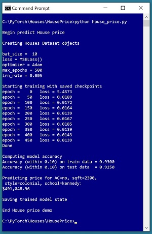 [Click on image for larger view.] Figure 1: Predicting the Price of a House Using Neural Regression
The demo trains the neural network for 500 epochs in batches of 10 items. An epoch is one complete pass through the training data. The training data has 200 items, therefore, one training epoch consists of processing 20 batches of 10 training items.
During training, the demo computes and displays a measure of the current error (also called loss) every 50 epochs. Because error slowly decreases, it appears that training is succeeding. Behind the scenes, the demo program saves checkpoint information after every 50 epochs so that if the training machine crashes, training can be resumed without having to start over from the beginning.
After training the network, the demo program computes the prediction accuracy of the model based on whether or not the predicted house price is within 10 percent of the true house price. The accuracy on the training data is 93.00 percent (186 out of 200 correct) and the accuracy on the test data is 92.50 percent (37 out of 40 correct). Because the two accuracy values are similar, it is likely that model overfitting has not occurred.
Next, the demo uses the trained model to make a prediction on a new, previously unseen house. The raw input is (air conditioning = "no", square feet area = 2300, style = "colonial", school = "kennedy"). The raw input is normalized and encoded as (air conditioning = -1, area = 0.2300, style = 0,0,1, school = 0,1,0). The computed output price is 0.49104896 which is equivalent to $491,048.96 because the raw house prices were all normalized by dividing by 1,000,000.
The demo program concludes by saving the trained model using the state dictionary approach. This is the most common of three standard techniques.
This article assumes you have an intermediate or better familiarity with a C-family programming language, preferably Python, but doesn't assume you know very much about PyTorch. The complete source code for the demo program, and the two data files used, are available in the download that accompanies this article. All normal error checking code has been omitted to keep the main ideas as clear as possible.
To run the demo program, you must have Python and PyTorch installed on your machine. The demo programs were developed on Windows 10 using the Anaconda 2020.02 64-bit distribution (which contains Python 3.7.6) and PyTorch version 1.7.0 for CPU installed via pip. You can find detailed step-by-step installation instructions for this configuration in my blog post.
The House Data
The raw House data is synthetic and was generated programmatically. There are a total of 240 data items, divided into a 200-item training dataset and a 40-item test dataset. The raw data looks like:
no    1275   bungalow   $318,000.00   lincoln
yes   1100   art_deco   $335,000.00   johnson
no    1375   colonial   $286,000.00   kennedy
yes   1975   bungalow   $512,000.00   lincoln
. . .
no    2725   art_deco   $626,000.00   kennedy
Each line of tab-delimited data represents one house. The value to predict, house price, is in 0-based column [3]. The predictors variables in columns [0], [1], [2] and [4] are air conditioning yes-no, area in square feet, architectural style and local school. For simplicity, there are just three house styles and three schools.
House area values were normalized by dividing by 10,000 and house prices were normalized by dividing by 1,000,000. Air conditioning was binary encoded as no = -1, yes = +1. Style was one-hot encoded as "art_deco" = (1,0,0), "bungalow" = (0,1,0), "colonial" = (0,0,1). School was one-hot encoded as "johnson" = (1,0,0), "kennedy" = (0,1,0), "lincoln" = (0,0,1). The resulting normalized and encoded data looks like:
-1   0.1275   0 1 0   0.3180   0 0 1
 1   0.1100   1 0 0   0.3350   1 0 0
-1   0.1375   0 0 1   0.2860   0 1 0
 1   0.1975   0 1 0   0.5120   0 0 1
. . .
-1   0.2725   1 0 0   0.6260   0 1 0
After the structure of the training and test files was established, I designed and coded a PyTorch Dataset class to read the house data into memory and serve the data up in batches using a PyTorch DataLoader object. A Dataset class definition for the normalized and encoded House data is shown in Listing 1.
Listing 1: A Dataset Class for the Student Data
class HouseDataset(T.utils.data.Dataset):
  # AC  sq ft   style  price   school
  # -1  0.2500  0 1 0  0.5650  0 1 0
  #  1  0.1275  1 0 0  0.3710  0 0 1
  # air condition: -1 = no, +1 = yes
  # style: art_deco, bungalow, colonial
  # school: johnson, kennedy, lincoln

  def __init__(self, src_file, m_rows=None):
    all_xy = np.loadtxt(src_file, max_rows=m_rows,
      usecols=[0,1,2,3,4,5,6,7,8], delimiter="\t",
      comments="#", skiprows=0, dtype=np.float32)

    tmp_x = all_xy[:,[0,1,2,3,4,6,7,8]]
    tmp_y = all_xy[:,5].reshape(-1,1)    # 2-D

    self.x_data = T.tensor(tmp_x, \
      dtype=T.float32).to(device)
    self.y_data = T.tensor(tmp_y, \
      dtype=T.float32).to(device)

  def __len__(self):
    return len(self.x_data)

  def __getitem__(self, idx):
    preds = self.x_data[idx,:]  # or just [idx]
    price = self.y_data[idx,:]
    return (preds, price)       # tuple of matrices
Preparing data and defining a PyTorch Dataset is not trivial. You can find the article that explains how to create Dataset objects and use them with DataLoader objects here.
The Neural Network Architecture
In the previous article in this series, I described how to design and implement a neural network for regression for the House data. One possible definition is presented in Listing 2. The code defines an 8-(10-10)-3 neural network with relu() activation on the hidden nodes.
Listing 2: A Neural Network for the Student Data
class Net(T.nn.Module):
  def __init__(self):
    super(Net, self).__init__()
    self.hid1 = T.nn.Linear(8, 10)  # 8-(10-10)-1
    self.hid2 = T.nn.Linear(10, 10)
    self.oupt = T.nn.Linear(10, 1)

    T.nn.init.xavier_uniform_(self.hid1.weight)
    T.nn.init.zeros_(self.hid1.bias)
    T.nn.init.xavier_uniform_(self.hid2.weight)
    T.nn.init.zeros_(self.hid2.bias)
    T.nn.init.xavier_uniform_(self.oupt.weight)
    T.nn.init.zeros_(self.oupt.bias)

  def forward(self, x):
    z = T.relu(self.hid1(x))
    z = T.relu(self.hid2(z))
    z = self.oupt(z)  # no activation
    return z
If you are new to PyTorch, the number of design decisions for a neural network can seem intimidating. But with every program you write, you learn which design decisions are important and which don't affect the final prediction model very much, and the pieces of the design puzzle eventually fall into place.
The Overall Program Structure
The overall structure of the PyTorch neural regression program, with a few minor edits to save space, is shown in Listing 3. I prefer to indent my Python programs using two spaces rather than the more common four spaces.
Listing 3: The Structure of the Demo Program
# house_price.py
# PyTorch 1.7.0-CPU Anaconda3-2020.02
# Python 3.7.6 Windows 10

import numpy as np
import time
import torch as T
device = T.device("cpu")

class HouseDataset(T.utils.data.Dataset):
  # AC  sq ft   style  price   school
  # -1  0.2500  0 1 0  0.5650  0 1 0
  #  1  0.1275  1 0 0  0.3710  0 0 1
  # air condition: -1 = no, +1 = yes
  # style: art_deco, bungalow, colonial
  # school: johnson, kennedy, lincoln

  def __init__(self, src_file, m_rows=None): . . .
  def __len__(self): . . .
  def __getitem__(self, idx): . . .

# ----------------------------------------------------

def accuracy(model, ds): . . .

# ----------------------------------------------------

class Net(T.nn.Module):
  def __init__(self): . . .
  def forward(self, x): . . .

# ----------------------------------------------------

def main():
  # 0. get started
  print("Begin predict House price ")
  T.manual_seed(4)
  np.random.seed(4)

  # 1. create Dataset and DataLoader objects
  # 2. create neural network
  # 3. train network
  # 4. evaluate model
  # 5. make a prediction
  # 6. save model
  print("End House price demo ")

if __name__== "__main__":
  main()
It's important to document the versions of Python and PyTorch being used because both systems are under continuous development. Dealing with versioning incompatibilities is a significant headache when working with PyTorch and is something you should not underestimate.
I like to use "T" as the top-level alias for the torch package. Most of my colleagues don't use a top-level alias and spell out "torch" many of times per program. Also, I use the full form of sub-packages rather than supplying aliases such as "import torch.nn.functional as functional." In my opinion, using the full form is easier to understand and less error-prone than using many aliases.
The demo program defines a program-scope CPU device object. I usually develop my PyTorch programs on a desktop CPU machine. After I get that version working, converting to a CUDA GPU system only requires changing the global device object to T.device("cuda") plus a minor amount of debugging.
The demo program defines just one helper method, accuracy(). All of the rest of the program control logic is contained in a single main() function. It is possible to define other helper functions such as train_net(), evaluate_model() and save_model(), but in my opinion this modularization approach unexpectedly makes the program more difficult to understand rather than easier to understand.
Training the Neural Network
The details of training a neural network with PyTorch are complicated but the code is relatively simple. In very high-level pseudo-code, the process to train a neural network looks like:
    loop max_epochs times
      loop thru all batches of train data
        read a batch of data (inputs, targets)
        compute outputs using the inputs
        compute error between outputs and targets
        use error to update weights and biases
      end-loop (all batches)
    end-loop (all epochs)
The difficult part of training is the "use error to update weights and biases" step. PyTorch does most, but not all, of the hard work for you. It's not easy to understand neural network training without seeing a working program. The test program shown in Listing 4 demonstrates how to train a network for multi-class classification. The screenshot in Figure 2 shows the output from the test program.
Listing 4: Testing Neural Network Training Code
# test_training.py

import numpy as np
import time
import torch as T
device = T.device("cpu")

class HouseDataset(T.utils.data.Dataset):
  def __init__(self, src_file, m_rows=None):
    all_xy = np.loadtxt(src_file, max_rows=m_rows,
      usecols=[0,1,2,3,4,5,6,7,8], delimiter="\t",
      comments="#", skiprows=0, dtype=np.float32)

    tmp_x = all_xy[:,[0,1,2,3,4,6,7,8]]
    tmp_y = all_xy[:,5].reshape(-1,1)    # 2-D

    self.x_data = T.tensor(tmp_x, \
      dtype=T.float32).to(device)
    self.y_data = T.tensor(tmp_y, \
      dtype=T.float32).to(device)

  def __len__(self):
    return len(self.x_data)

  def __getitem__(self, idx):
    preds = self.x_data[idx,:]  # or just [idx]
    price = self.y_data[idx,:]
    return (preds, price)       # tuple of matrices

class Net(T.nn.Module):
  def __init__(self):
    super(Net, self).__init__()
    self.hid1 = T.nn.Linear(8, 10)  # 8-(10-10)-1
    self.hid2 = T.nn.Linear(10, 10)
    self.oupt = T.nn.Linear(10, 1)

    T.nn.init.xavier_uniform_(self.hid1.weight)
    T.nn.init.zeros_(self.hid1.bias)
    T.nn.init.xavier_uniform_(self.hid2.weight)
    T.nn.init.zeros_(self.hid2.bias)
    T.nn.init.xavier_uniform_(self.oupt.weight)
    T.nn.init.zeros_(self.oupt.bias)

  def forward(self, x):
    z = T.relu(self.hid1(x))
    z = T.relu(self.hid2(z))
    z = self.oupt(z)  # no activation
    return z

print("\nBegin test of training code\n")

T.manual_seed(1)
np.random.seed(1)
train_file = ".\\Data\\houses_train.txt"
train_ds = HouseDataset(train_file, m_rows=200)

bat_size = 10
train_ldr = T.utils.data.DataLoader(train_ds,
  batch_size=bat_size, shuffle=True)

net = Net().to(device)
net.train()  # set mode

lrn_rate = 0.005
loss_func = T.nn.MSELoss()
optimizer = T.optim.Adam(net.parameters(),
  lr=lrn_rate)

for epoch in range(0, 500):
  # T.manual_seed(1 + epoch)  # recovery reproduce
  epoch_loss = 0.0  # sum avg loss per item

  for (batch_idx, batch) in enumerate(train_ldr):
    X = batch[0]  # predictors shape [10,8]
    Y = batch[1]  # targets shape [10,1]

    optimizer.zero_grad()
    oupt = net(X)            # shape [10,1]

    loss_val = loss_func(oupt, Y)  # avg loss in batch
    epoch_loss += loss_val.item()  # a sum of averages
    loss_val.backward()
    optimizer.step()

  if epoch % 100 == 0:
    print(" epoch = %4d   loss = %0.4f" % \
     (epoch, epoch_loss))
    # TODO: save checkpoint

print("\nDone ")