The Data Science Lab

Quantum-Inspired Annealing Using C# or Python

Dr. James McCaffrey of Microsoft Research explains a new idea that slightly modifies standard simulated annealing by borrowing ideas from quantum mechanics.

• By James McCaffrey
• 01/20/2022

The goal of a combinatorial optimization problem is to find the best ordering of a set of discrete items. A classic combinatorial optimization challenge is the Traveling Salesman Problem (TSP). For TSP, you want to find the order in which to visit a set of cities so that the total distance traveled is minimized.

One of the oldest and simplest techniques for solving combinatorial optimization problems is called simulated annealing. A relatively new idea is to slightly modify standard simulated annealing by borrowing one or more ideas from quantum mechanics. This is sometimes called quantum-inspired annealing. Note that quantum-inspired algorithms do not use quantum computing hardware. Quantum-inspired algorithms are just modifications of existing classical algorithms, and they run on standard hardware.

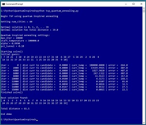
A good way to see where this article is headed is to take a look at the screenshot of a demo program in Figure 1. The demo sets up a synthetic problem where there are 40 cities, labeled 0 through 39. The distance between cities is designed so that the best route starts at city 0 and then visits each city in order. The total distance of the optimal route is 39.0.

The demo sets up quantum-inspired annealing parameters of max_iter = 20_000, start_temperature = 100_000.0, alpha = 0.9990, and pct_tunnel = 0.10. Quantum-inspired annealing is an iterative process and max_iter is the maximum number of times the processing loop will execute. The start_temperature and alpha parameters control how the classical part of the annealing algorithm explores possible solution routes. The pct_tunnel parameter controls how often the quantum-inspired part of the algorithm is used.

The demo sets up a random initial guess of the best route as [ 7, 34, 21 . . 9, 10 ]. After iterating 20,000 times, the demo reports the best route found as [ 0, 1, 2, 3, 4, 5, 6, 7, 8, 9, 16, 19, 18, 15, 14, 13, 12, 10, 11, 17, 20, 21, 22, 23, 24, 25, 26, 27, 28, 29, 30, 31, 32, 33, 34, 35, 36, 37, 38, 39 ]. The total distance required to visit the cities in this order is 61.5 and so the solution is close to, but not quite as good as, the optimal solution. The first 10 cities and the last 20 cities are visited in correct order but the middle 10 cities are not visited correctly.

This article assumes you have an intermediate or better familiarity with a C-family programming language, preferably C# or Python, but does not assume you know anything about simulated annealing. The complete source code for the demo program is presented in this article, and the code is also available in the accompanying file download.

Understanding Classical Simulated Annealing
Quantum-inspired annealing is a slight adaptation of classical simulated annealing. Suppose you have a combinatorial optimization problem with just five elements, and where the best ordering/permutation is [B, A, D, C, E]. A primitive approach would be to start with a random permutation such as [C, A, E, B, D] and then repeatedly swap randomly selected pairs of elements until you find the best ordering. For example, if you swap the elements at [0] and [1], the new permutation is [A, C, E, B, D]. You'd repeat generating new permutations until you found a good result.

This brute force approach works if there are just a few elements in the problem permutation, but fails for even a moderate number of elements. For the demo problem with n = 40 cities, there are 40! possible permutations = 40 * 39 * 38 * . . * 1 = 815,915,283,247,897,734,345,611,269,596,115,894,272,000,000,000. Even if you could examine one billion candidate solutions per second, to check all permutations would take you roughly 9,000,000,000,000,000,000,000,000,000,000,000 years, which is much longer than the estimated age of the universe (about 14,000,000,000 years).

To understand quantum-inspired annealing you must first understand classical simulated annealing. Expressed as pseudo-code, classical simulated annealing is:

make a random initial guess permutation
  set a large initial temperature
  loop many times
    swap two randomly selected elements of the curr guess
    compute error of proposed candidate solution
    if proposed solution is better than curr solution then
      accept the proposed solution
    else if proposed solution is worse then
      sometimes accept solution anyway, based on curr temp
    end-if
    decrease temperature value slightly
  end-loop
  return best solution found

By swapping two randomly selected elements of the current solution, an adjacent proposed solution is created. The adjacent proposed solution will be similar to the current guess so the search process isn't completely random. A good current solution will likely lead to a good new proposed solution.

By sometimes accepting a proposed solution that's worse than the current guess, you can avoid getting trapped into a good but not optimal solution. The probability of accepting a worse solution is given by:

accept_p = exp((err - adj_err) / curr_temperature)

where exp() the mathematical exp() function, err is the error associated with the current guess, adj_err is the error associated with the proposed adjacent solution, and curr_temperature is a value such as 1000.0.

In simulated annealing, the temperature value starts out large, such as 1000000.0 and then is reduced slowly on each iteration. Early in the algorithm, when temperature is large, accept_p will be large (close to 1) and the algorithm will often move to a worse solution. This allows many permutations to be examined. Late in the algorithm, when temperature is small, accept_p will be small (close to 0) and the algorithm will rarely move to a worse solution.

The temperature reduction is controlled by the alpha value. Suppose the current temperature = 1000.0 and alpha = 0.90. After the next processing iteration, temperature becomes 1000.0 * 0.90 = 900.0. After the next iteration temperature becomes 900.0 * 0.90 = 810.0. After a third iteration temperature becomes 810.0 * 0.90 = 729.0. And so on. Smaller values of alpha decrease temperature more quickly.

Adding Quantum Inspired Tunneling
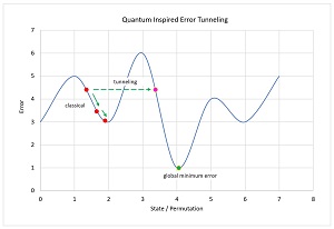
Quantum-inspired annealing adds a slight twist to classical simulated annealing. In quantum mechanics there is an idea called quantum tunneling. Briefly, and very loosely, a quantum particle will usually transition from its current energy state to an adjacent lower energy state. When a particle encounters a potential barrier it will usually be blocked, but will sometimes tunnel through the barrier to a non-adjacent state.

This quantum tunneling can be used to improve classical simulated annealing. The key ideas are shown in the graph in Figure 2. In classical simulated annealing for TSP, the states are permutations of cities. If you transition only from the current state to an adjacent state (when the order of only one pair of cities is changed), you can get stuck at a local minimum error. If you allow tunneling, you can take a large jump to escape and get back on track to find the state with the global minimum error.

So, quantum-inspired tunneling just means sometimes allowing a candidate solution to be farther away from the current solution. This can be achieved by swapping more than just two cities. For example, if you swap 10 pairs of randomly selected cities, the result permutation will be father away from the source permutation than if you swap just one pair of randomly selected cities.

Early in the algorithm, when creating a candidate solution, you can swap many pairs of cities, generating a candidate that is far from the current permutation. Later in the algorithm you swap fewer pairs of cities. Expressed in pseudo-code:

set pct_tunnel (like 0.10)
  loop many times
    p = random in [0.0, 1.0)
    if p < pct_tunnel then (do tunneling)
      set num_swaps = large, based on pct iterations left
    else
      set num_swaps = 1 (no tunneling)
    end-if
    create candidate solution using num_swaps
    apply classical annealing
  end-loop
  return best solution found

The Python version of the function that creates a candidate permutation-solution is:

def adjacent(route, n_swaps, rnd):
  n = len(route)
  result = np.copy(route)
  for ns in range(n_swaps):
    i = rnd.randint(n)
    j = rnd.randint(n)
    tmp = result[i]
    result[i] = result[j]
    result[j] = tmp
  return result

The route parameter is the current solution. The n_swaps parameter specifies how many pair of cities to swap when creating the candidate solution. The rnd parameter is a local random number generator object.

An equivalent C# version of the function is:

static int[] Adjacent(int[] route, int numSwaps, Random rnd)
{
  int n = route.Length;
  int[] result = (int[])route.Clone();
  for (int ns = 0; ns < numSwaps; ++ns) {
    int i = rnd.Next(0, n);
    int j = rnd.Next(0, n);
    int tmp = result[i];
    result[i] = result[j];
    result[j] = tmp;
  }
  return result;
}

The key parameter is the number of pairs of cities to swap. The demo program computes this as the percent of iterations remaining times the total number of cities. For example, for n = 40 cities, if max_iterations = 1000 and the current iteration is 300, then there are 700 / 1000 = 0.70 of the iterations remaining, and the number of swaps would be 0.70 * 40 = 28.

The Demo Program
The complete quantum-inspired annealing demo program using Python, with a few minor edits to save space, is presented in Listing 1. I indent using two spaces rather than the standard four spaces. The backslash character is used for line continuation to break down long statements. You can find an equivalent C# version of the demo program on my blog.

Listing 1: The Quantum Annealing for TSP Python Language Program

# tsp_quantum_annealing.py
# traveling salesman problem 
# quantum inspired simulated annealing
# Python 3.7.6 (Anaconda3 2020.02)

import numpy as np

def total_dist(route):
  d = 0.0  # total distance between cities
  n = len(route)
  for i in range(n-1):
    if route[i] < route[i+1]:
      d += (route[i+1] - route[i]) * 1.0
    else:
      d += (route[i] - route[i+1]) * 1.5
  return d

def error(route):
  n = len(route)
  d = total_dist(route)
  min_dist = n-1
  return d - min_dist

def adjacent(route, n_swaps, rnd):
  # tunnel if n_swaps > 1
  n = len(route)
  result = np.copy(route)
  for ns in range(n_swaps):
    i = rnd.randint(n); j = rnd.randint(n)
    tmp = result[i]
    result[i] = result[j]; result[j] = tmp
  return result

def my_kendall_tau_dist(p1, p2):
  # p1, p2 are 0-based lists or np.arrays
  n = len(p1)
  index_of = [None] * n  # lookup into p2
  for i in range(n):
    v = p2[i]; index_of[v] = i

  d = 0  # raw distance = number pair misorderings
  for i in range(n):
    for j in range(i+1, n):
      if index_of[p1[i]] > index_of[p1[j]]:
        d += 1
  normer = n * (n - 1) / 2.0
  nd = d / normer  # normalized distance
  return (d, nd) 

def solve_qa(n_cities, rnd, max_iter, start_temperature,
  alpha, pct_tunnel):
  curr_temperature = start_temperature
  soln = np.arange(n_cities, dtype=np.int64)  # [0,1,2, . . ]
  rnd.shuffle(soln)
  print("Initial guess: ")
  print(soln); print("")

  err = error(soln)
  iter = 0
  interval = (int)(max_iter / 10)
  num_swaps = n_cities

  best_soln = np.copy(soln)
  best_err = err

  while iter < max_iter and err > 0.0:
  # while iter < max_iter:
    # pct left determines n_swaps determines distance
    pct_iters_left = (max_iter - iter) / (max_iter * 1.0)
    if pct_iters_left < 0.00001: 
      pct_iters = 0.00001

    p = rnd.random()  # [0.0, 1.0]
    if p < pct_tunnel:  # tunnel
      num_swaps = (int)(pct_iters_left * n_cities)
      if num_swaps < 1:
        num_swaps = 1
    else:  # no tunneling
      num_swaps = 1

    adj_route = adjacent(soln, num_swaps, rnd)
    adj_err = error(adj_route)

    if adj_err < best_err:
      best_soln = np.copy(adj_route)
      best_err = adj_err

    if adj_err < err:  # better route so accept
      soln = adj_route; err = adj_err
    else:          # adjacent is worse
      accept_p = np.exp((err - adj_err) / curr_temperature)
      p = rnd.random()
      if p < accept_p:  # accept anyway
        soln = adj_route
        err = adj_err 
      # else don't accept worse route
   
    if iter % interval == 0:
      (dist, nd) = my_kendall_tau_dist(soln, adj_route)
      print("iter = %6d | " % iter, end="")
      print("dist curr to candidate = %8.4f | " \
        % nd, end="")
      print("curr_temp = %12.4f | " \
        % curr_temperature, end="")
      print("error = %6.1f " % best_err)

    if curr_temperature < 0.00001:
      curr_temperature = 0.00001
    else:
      curr_temperature *= alpha

    iter += 1
  return best_soln 

def main():
  print("\nBegin TSP using quantum inspired annealing ")

  num_cities = 40
  print("\nSetting num_cities = %d " % num_cities)
  print("\nOptimal solution is 0, 1, 2, . . " + \
    str(num_cities-1))
  print("Optimal solution has total distance = %0.1f " \
    % (num_cities-1))
  rnd = np.random.RandomState(6)
  max_iter = 20_000  # 120000 finds optimal solution
  start_temperature = 100_000.0
  alpha = 0.9990
  pct_tunnel = 0.10

  print("\nQuantum inspired annealing settings: ")
  print("max_iter = %d " % max_iter)
  print("start_temperature = %0.1f " \
    % start_temperature)
  print("alpha = %0.4f " % alpha)
  print("pct_tunnel = %0.2f " % pct_tunnel)

  print("\nStarting solve() ")
  soln = solve_qa(num_cities, rnd, max_iter, \
    start_temperature, alpha, pct_tunnel)
  print("Finished solve() ")

  print("\nBest solution found: ")
  print(soln)
  dist = total_dist(soln)
  print("\nTotal distance = %0.1f " % dist)

  print("\nEnd demo ")
if __name__ == "__main__":
  main()

• Get Code Download