The Data Science Lab
Multi-Class Classification Using a scikit Neural Network
Dr. James McCaffrey of Microsoft Research says a neural network model is arguably the most powerful multi-class classification technique.
A multi-class classification problem is one where the goal is to predict the value of a variable where there are three or more discrete possibilities. For example, you might want to predict the political leaning of a person (conservative = 0, moderate = 1, liberal = 2) based on their sex, age, state where they live and income. Note that when there are just two possible values to predict (for example, sex = male or female), the problem is called binary classification, which typically uses different algorithms.
Arguably the most powerful multi-class classification technique is a neural network model. There are several tools and code libraries that you can use to create a neural network classifier. The scikit-learn library (also called scikit or sklearn) is based on the Python language and is one of the most popular.
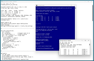
A good way to see where this article is headed is to take a look at the screenshot in Figure 1. The demo program loads a 200-item set of training data and a 40-item set of test data into memory. Next, the demo creates and trains a neural network model using the MLPClassifier module ("multi-layer perceptron," an old term for a neural network) from the scikit library.
 [Click on image for larger view.] Figure 1: Multi-Class Classification Using a scikit Neural Network
After training, the model is applied to the training data and the test data. The model scores 87.50 percent accuracy (175 out of 200 correct) on the training data, and 77.50 percent accuracy (31 out of 40 correct) on the test data.
The demo concludes by predicting the political leaning of a person who is male, age 35, from Nebraska and makes $55,000 per year. The prediction is [[0.0008 0.8293 0.1699]]. These are pseudo-probabilities and because the value at index [1] is largest, the predicted political type is moderate.
This article assumes you have intermediate or better skill with a C-family programming language, but doesn't assume you know much about neural networks or the scikit library. The complete source code for the demo program is presented in this article and the accompanying file download. The source code and training and test data are also available online.
Installing the scikit Library
There are several ways to install the scikit library. I recommend installing the Anaconda Python distribution. Anaconda contains a core Python engine plus more than 500 libraries that are (mostly) compatible with each other. I used Anaconda3-2020.02, which contains Python 3.7.6 and the scikit 0.22.1 version. The demo code runs on Windows 10 or 11.
Briefly, Anaconda is installed using a Windows self-extracting executable file. The setup process is mostly straightforward and takes about 15 minutes following my step-by-step instructions.
There are more up-to-date versions of Anaconda / Python / scikit library available. However, because the Python ecosystem has hundreds of libraries, if you install the most recent versions of these libraries, you run a greater risk of library incompatibilities -- a significant headache when working with Python.
The Data
The data is artificial. There are 200 training items and 40 test items. The structure of data looks like:
 1   0.24   1  0  0   0.2950   2
-1   0.39   0  0  1   0.5120   1
 1   0.63   0  1  0   0.7580   0
-1   0.36   1  0  0   0.4450   1
 1   0.27   0  1  0   0.2860   2
. . .
The tab-delimited fields are sex (-1 = male, 1 = female), age (divided by 100), state (Michigan = 100, Nebraska = 010, Oklahoma = 001), income (divided by $100,000) and political leaning (conservative = 0, moderate = 1, liberal = 2). For scikit neural network classification, the variable to predict is most often zero-based ordinal-encoded (0, 1, 2 and so on) The numeric predictors should be normalized to all the same range -- typically 0.0 to 1.0 or -1.0 to +1.0 -- as normalizing prevents predictors with large magnitudes from overwhelming those with small magnitudes.
For categorical predictor variables, I recommend one-hot encoding. For example, if there were five states instead of just three, the states would be encoded as 10000, 01000, 00100, 00010, 00001. For binary predictor variables, such as sex, you can encode using either zero-one encoding or minus-one-plus-one encoding. The demo uses minus-one-plus-one encoding. In spite of decades of research, there are some topics, such as binary predictor encoding, that are not well understood (see my article, "Encoding Binary Predictor Variables for Neural Networks").
The Demo Program
The complete demo program is presented in Listing 1. Notepad is my preferred code editor but most of my colleagues favor one of the many excellent code editors that are available for Python. I indent my Python program using two spaces rather than the more common four spaces.
The program imports the NumPy library, which contains numeric array functionality, and the MLPClassifier module, which contains neural network functionality. Notice the name of the root scikit module is sklearn rather than scikit.
import numpy as np
from sklearn.neural_network import MLPClassifier
import warnings
warnings.filterwarnings('ignore')  # early-stop warnings
The demo specifies that no Python warnings should be displayed. I do this to keep the output tidy, but in a non-demo scenario you definitely want to see warning messages.
Listing 1:
Complete Demo Program
# people_politics_nn_sckit.py

# predict political leaning
# from sex, age, state, income

# sex  age    state    income   politics
# -1   0.27   0 1 0    0.7610   2
#  1   0.19   0 0 1    0.6550   0
# sex: -1 = male, 1 = female
# state: michigan = 100, nebraska = 010, oklahoma = 001
# politics: conservative = 0, moderate = 1, liberal = 2

# Anaconda3-2020.02  Python 3.7.6  scikit 0.22.1
# Windows 10/11

import numpy as np
from sklearn.neural_network import MLPClassifier
import warnings
warnings.filterwarnings('ignore')  # early-stop warnings

# ---------------------------------------------------------

def main():
  # 0. get ready
  print("\nBegin scikit neural network example ")
  print("Predict politics from sex, age, State, income ")
  np.random.seed(1)
  np.set_printoptions(precision=4, suppress=True)

  # sex  age    state    income   politics
  # -1   0.27   0 1 0    0.7610   2
  #  1   0.19   0 0 1    0.6550   0

  # 1. load data
  print("\nLoading data into memory ")
  train_file = ".\\Data\\people_train.txt"
  train_xy = np.loadtxt(train_file, usecols=range(0,7),
    delimiter="\t", comments="#",  dtype=np.float32)
  train_x = train_xy[:,0:6]
  train_y = train_xy[:,6].astype(int)

  test_file = ".\\Data\\people_test.txt"
  test_xy = np.loadtxt(test_file, usecols=range(0,7),
    delimiter="\t", comments="#",  dtype=np.float32)
  test_x = test_xy[:,0:6]
  test_y = test_xy[:,6].astype(int)

  print("\nTraining data:")
  print(train_x[0:4])
  print(". . . \n")
  print(train_y[0:4])
  print(". . . ")

# ---------------------------------------------------------

  # 2. create network
  # MLPClassifier(hidden_layer_sizes=(100,),
  #  activation='relu', *, solver='adam', alpha=0.0001,
  #  batch_size='auto', learning_rate='constant',
  #  learning_rate_init=0.001, power_t=0.5, max_iter=200,
  #  shuffle=True, random_state=None, tol=0.0001,
  #  verbose=False, warm_start=False, momentum=0.9,
  #  nesterovs_momentum=True, early_stopping=False,
  #  validation_fraction=0.1, beta_1=0.9, beta_2=0.999,
  #  epsilon=1e-08, n_iter_no_change=10, max_fun=15000)

  params = { 'hidden_layer_sizes' : [10,10],
    'activation' : 'tanh',
    'solver' : 'sgd',
    'alpha' : 0.0,
    'batch_size' : 10,
    'random_state' : 1,
    'tol' : 0.0001,
    'nesterovs_momentum' : False,
    'learning_rate' : 'constant',
    'learning_rate_init' : 0.01,
    'max_iter' : 1000,
    'shuffle' : True,
    'n_iter_no_change' : 90,
    'verbose' : False }

  print("\nCreating 6-(10-10)-3 tanh neural network ")
  net = MLPClassifier(**params)

# ---------------------------------------------------------

  # 3. train
  print("\nTraining with bat sz = " + \
    str(params['batch_size']) + " lrn rate = " + \
    str(params['learning_rate_init']) + " ")
  print("Stop if no change " + \
    str(params['n_iter_no_change']) + " iterations ")
  net.fit(train_x, train_y)
  print("Done ")

  # 4. evaluate
  acc_train = net.score(train_x, train_y)
  print("\nAccuracy on train = %0.4f " % acc_train)
  acc_test = net.score(test_x, test_y)
  print("Accuracy on test = %0.4f " % acc_test)

  # 5. use model
  print("\nPredict for: M 35 Nebraska $55K ")
  X = np.array([[-1, 0.35, 0,1,0, 0.5500]],
    dtype=np.float32)

  probs = net.predict_proba(X)
  print("\nPrediction pseudo-probs: ")
  print(probs)

  politic = net.predict(X)  # 0,1,2
  lbls = ["conservative", "moderate", "liberal"]
  print("\nPredicted class: ")
  print(lbls[politic[0]])

  # 6. TODO: save model using pickle

  print("\nEnd scikit neural network demo ")

if __name__ == "__main__":
  main()
All the program logic is contained in a main() function. The demo begins by setting the NumPy random seed:
def main():
  # 0. get ready
  print("Begin scikit neural network example ")
  print("Predict politics from sex, age, State, income ")
  np.random.seed(1)
  np.set_printoptions(precision=4, suppress=True)
 . . .
Technically, setting the random seed value isn't necessary, but doing so helps you to get reproducible results in most situations. The set_printoptions() function formats NumPy arrays to four decimals without using scientific notation.
Loading the Training and Test Data
The demo program loads the training data into memory using these statements:
  # 1. load data
  print("Loading data into memory ")
  train_file = ".\\Data\\people_train.txt"
  train_xy = np.loadtxt(train_file, usecols=range(0,7),
    delimiter="\t", comments="#",  dtype=np.float32)
  train_x = train_xy[:,0:6]
  train_y = train_xy[:,6].astype(int)
This code assumes the data files are stored in a directory named Data. There are many ways to load data into memory. I prefer using the NumPy library loadtxt() function, but a common alternative is the Pandas library read_csv() function.
The code reads all 200 lines of training data (columns 0 to 6 inclusive) into a matrix named train_xy and then splits the data into a matrix of predictor values and a vector of target gender values. The colon syntax means "all rows." The labels (political leaning values) are converted from type float32 to int64.
The 40-item test data is read into memory in the same way as the training data:
  test_file = ".\\Data\\people_test.txt"
  test_xy = np.loadtxt(test_file, usecols=range(0,7),
    delimiter="\t", comments="#",  dtype=np.float32)
  test_x = test_xy[:,0:6]
  test_y = test_xy[:,6].astype(int)
The demo program prints the first four predictor items and the first four target politics values:
  print("Training data:")
  print(train_x[0:4])
  print(". . . \n")
  print(train_y[0:4])
  print(". . . ")
In a non-demo scenario you might want to display all the training data and all the test data to verify the data has been read properly.
Creating the Neural Network Model
Creating the multi-class classification neural network model is simultaneously simple and complicated. First, the demo program sets up the network parameters in a Python Dictionary object like so:
  # 2. create network
  params = { 'hidden_layer_sizes' : [10,10],
    'activation' : 'tanh', 'solver' : 'sgd',
    'alpha' : 0.0, 'batch_size' : 10,
    'random_state' : 1,'tol' : 0.0001,
    'nesterovs_momentum' : False,
    'learning_rate' : 'constant',
    'learning_rate_init' : 0.01,
    'max_iter' : 1000, 'shuffle' : True,
    'n_iter_no_change' : 90, 'verbose' : False }
After the parameters are set, they are fed to a neural network constructor:
  print("Creating 6-(10-10)-3 tanh neural network ")
  net = MLPClassifier(**params)
The ** syntax means to unpack the Dictionary values and pass them to the constructor. Like many scikit models, the MLPClassifier class has a lot of parameters and default values. The signature is:
MLPClassifier(hidden_layer_sizes=(100,),
 activation='relu', *, solver='adam', alpha=0.0001,
 batch_size='auto', learning_rate='constant',
 learning_rate_init=0.001, power_t=0.5, max_iter=200,
 shuffle=True, random_state=None, tol=0.0001,
 verbose=False, warm_start=False, momentum=0.9,
 nesterovs_momentum=True, early_stopping=False,
 validation_fraction=0.1, beta_1=0.9, beta_2=0.999,
 epsilon=1e-08, n_iter_no_change=10, max_fun=15000)
When working with scikit, you'll spend most of your time reading the documentation and trying to figure out what each parameter does. The MLPClassifier class is especially complex because many of the parameters interact with each other.
Your first parameter decision is the solver to use for training the network. Your choices are 'adam', 'sgd', or 'lbfgs'. I recommend 'sgd' for most problems, even though 'adam' is the default. The 'adam' solver is essentially a sophisticated version of 'sgd'. The 'lbfgs' solver works in a completely different way from 'adam' and 'sgd'.
Your next parameter decision is the number of hidden layers and the number of processing nodes in each layer. The demo uses two hidden layers with 10 nodes each. More layers and more nodes are not always better, so you must experiment. The default is one hidden layer with 100 nodes.